I read Designing Machine Learning Systems: An Iterative Process for Production-Ready Applications by Chip Huyen on August 12, 2026

Contents

1. Chapter 1. Overview of Machine Learning Systems
2. Chapter 2. Introduction to Machine Learning Systems Design
3. Chapter 3. Data Engineering Fundamentals
4. Chapter 4. Training Data
5. Chapter 5. Feature Engineering
6. Chapter 6. Model Development and Offline Evaluation
7. Chapter 7. Model Deployment and Prediction Service
8. Chapter 8. Data Distribution Shifts and Monitoring
9. Chapter 9. Continual Learning and Test in Production
10. Chapter 10. Infrastructure and Tooling for MLOps
11. Chapter 11. The Human Side of Machine Learning

The preface goes over how Chip started this book which was from writing down and preparing classes for her Machine Learning students back in 2017 and how similar where the questions shed had like:

“What model should I use?” “How often should I retrain my model?” “How can I detect data distribution shifts?” “How do I ensure that the features used during training are consistent with the features used during inference?”

ML systems are both complex and unique. They are complex because they consist of many different components (ML algorithms, data, business logic, evaluation metrics, underlying infrastructure, etc.) and involve many different stakeholders (data scientists, ML engineers, business leaders, users, even society at large). ML systems are unique because they are data dependent, and data varies wildly from one use case to the next.

For example, two companies might be in the same domain (ecommerce) and have the same problem that they want ML to solve (recommender system), but their resulting ML systems can have different model architecture, use different sets of features, be evaluated on different metrics, and bring different returns on investment.

Chapter 1. Overview of Machine Learning Systems

In November 2016, Google announced that it had incorporated its multilingual neural machine translation system into Google Translate, marking one of the first success stories of deep artificial neural networks in production at scale. According to Google, with this update, the quality of translation improved more in a single leap than they had seen in the previous 10 years combined.

Many people, when they hear “machine learning system,” think of just the ML algorithms being used such as logistic regression or different types of neural networks.

However, the algorithm is only a small part of an ML system in production. The system also includes the business requirements that gave birth to the ML project in the first place, the interface where users and developers interact with your system, the data stack, and the logic for developing, monitoring, and updating your models, as well as the infrastructure that enables the delivery of that logic.

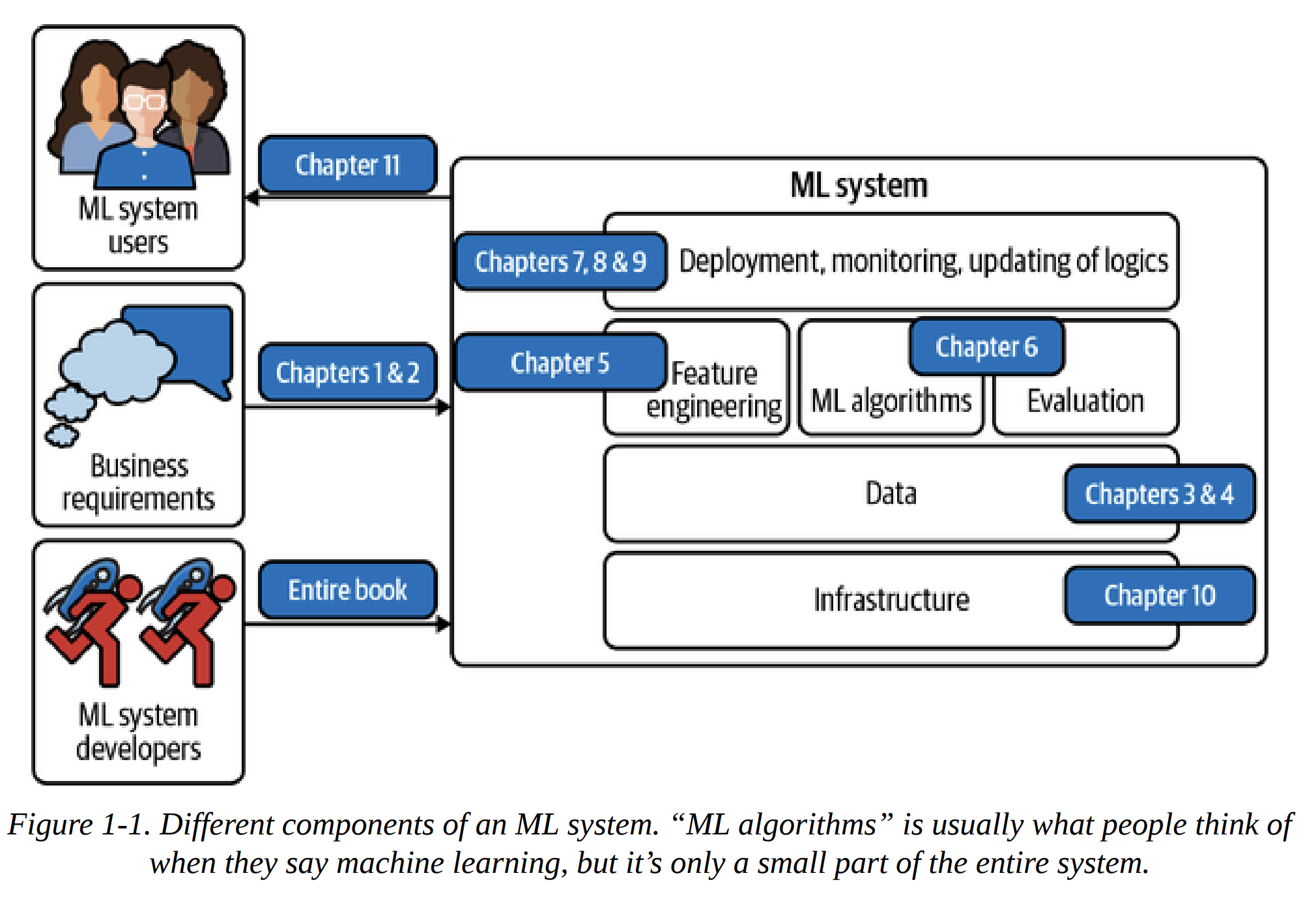
Before discussing how to develop an ML system, it’s important to ask a fundamental question of when and when not to use ML.

After the use cases, we’ll move on to the challenges of deploying ML systems, and we’ll do so by comparing ML in production to ML in research as well as to traditional software.

When to Use Machine Learning.

ML has proven to be a powerful tool for a wide range of problems. Despite an incredible amount of excitement and hype generated by people both inside and outside the field, ML is not a magic tool that can solve all problems. Even for problems that ML can solve, ML solutions might not be the optimal solutions. Before starting an ML project, you might want to ask whether ML is necessary or cost-effective.

ML solutions generally do:

Machine learning is an approach to (1) learn (2) complex patterns from (3) existing data and use these patterns to make (4) predictions on (5) unseen data.

1. Learn: the system has the capacity to learn.

Example: a relational databse can have a relationship between 2 tables but it doesn’t find it by its own, you need to define and tell the system that there’s a link, on the other hand a ML system learns and figure out that relationship.

1. Complex patterns: there are patterns to learn, and they are complex.

Whether a pattern exists might not be obvious, or if patterns exist, your dataset or ML algorithms might not be sufficient to capture them.

Example: you can train a ML model on how Elon Musk’s tweets affect crypto currencies prices. Or given a zip code and some characteristics provide an Airbnb price. What is complex to machines is different from what is complex to humans.

Given these features, ML is also called Software 2.0.

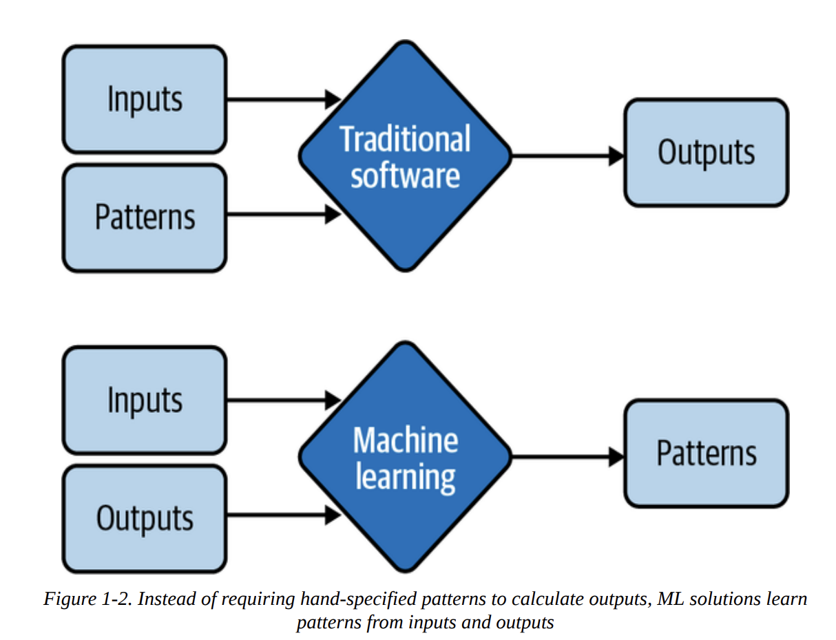
1. Existing data: data is available, or it’s possible to collect data.

Example: if we want to predict how much taxes a person will pay next year, we must have access to data like taxes and income.

Another approach is to launch a model (within a product) and let the user use it and while the usage carries on we capture that new data.

1. Predictions: it’s a predictive problem.

ML models make predictions, so they can only solve problems that require predictive answers.

Example: what will the weather be like tomorrow? Who will win the Super Bowl this year? What movie will a user want to watch next?

1. Unseen data: unseen data shares patterns with the training data.

The patterns your model learns from existing data are only useful if unseen data also share these patterns.

In technical terms, it means your unseen data and training data should come from similar distributions.

Example: a model to predict wheter an app will be downloaded on Xmas 2025 wont perform well if it’s been trained on 2008 data.

These ML systems need additional characteristics:

• It’s repetitive.

ML algorithms still require many examples to learn a pattern.

• The cost of wrong predictions is cheap.

Example: a recommeder system can not get user click but that’s not catastrophic as a self-driving car going over the sidewalk.

The benefits of correct predictions outweigh the cost of wrong predictions.

• It’s at scale.

Having a problem at scale also means that there’s a lot of data for you to collect, which is useful for training ML models.

Example: who will win US elections.

• The patterns are constantly changing.

Example: the email spam from a Nigerian Prince is well known, and if we have hardcoded rules once the spam changes we will fail to catch the fraud, therefore since ML system learns from data, you can update your ML model with new data without having to figure out how the data has changed.

Machine Learning Use Cases

Starting in 2010 there has been a boom of new ML cases on both, enterprise and consumer applications. They share some conditions and also differ on requirements like latency, optimization, investment and the usage can go widely from cost reduction, generating customer insights, improving customer experience, price optimization to internal automation.

Fraud detection is among the oldest applications of ML in the enterprise world. By leveraging ML solutions for anomaly detection, you can have systems that learn from historical fraud transactions and predict whether a future transaction is fraudulent.

Example: Acquiring a new user is expensive. Reducing customer acquisition costs by a small amount can result in a large increase in profit. This can be done through better identifying potential customers, showing better-targeted ads, giving discounts at the right time, etc. All of which are suitable tasks for ML.

After you’ve spent so much money acquiring a customer, it’d be a shame if they leave. To prevent customers from leaving, it’s important to keep them happy by addressing their concerns as soon as they arise. Automated support ticket classification can help with that.

An ML system can analyze the ticket content and predict where it should go, which can shorten the response time and improve customer satisfaction.

A set of ML use cases that has generated much excitement recently is in health care. There are ML systems that can detect skin cancer and diagnose diabetes.

Understanding Machine Learning Systems.

Machine Learning in Research Versus in Production.

The practice that is gain in research is very different that the one you gain in tech companies.

In research you seek state-of-the-art model performance, fast training, data is static and on the other hand with companies we have different stakeholders, different targets, user needs low latency, fast inference.

Example of a restaurant recommendation system:

                        RESTAURANT
                     RECOMMENDATION
                         SYSTEM
                            |
        ┌───────────┬───────┼──────────┬─────────────┐
        ↓           ↓       ↓          ↓             ↓
   ML Engineers   Sales   Product   ML Platform    Manager
        |           |       |          |             |
        ↓           ↓       ↓          ↓             ↓
 Maximize model   Higher   <100 ms   Reliability   Maximize
   accuracy /     priced   latency     + scale      margin
 relevance        places

ML Engineers → more data + complexity
Sales        → more service-fee revenue
Product      → low latency → more completed orders
ML Platform  → fewer updates → system stability
Manager      → lower costs / higher profit

“Recommending the restaurants that users are most likely to click on” and “recommending the restaurants that will bring in the most money for the app” are two different objectives

Computational priorities.

During the model development process, you might train many different models, and each model does multiple passes over the training data. Each trained model then generates predictions on the validation data once to report the scores. The validation data is usually much smaller than the training data.

During model development, training is the bottleneck. Once the model has been deployed, however, its job is to generate predictions, so inference is the bottleneck.

To reduce latency in production, you might have to reduce the number of queries you can process on the same hardware at a time. If your hardware is capable of processing many more queries at a time, using it to process fewer queries means underutilizing your hardware, increasing the cost of processing each query

When thinking about latency, it’s important to keep in mind that latency is not an individual number but a distribution.

Data

During the research phase, the datasets you work with are often clean and well-formatted, freeing you to focus on developing models. They are static by nature so that the community can use them to benchmark new architectures and techniques.

In production, data, if available, is a lot more messy. It’s noisy, possibly unstructured, constantly shifting.

Fairness

During the research phase, a model is not yet used on people, so it’s easy for researchers to put off fairness as an afterthought: “Let’s try to get state of the art first and worry about fairness when we get to production.” When it gets to production, it’s too late.

There’s no equivalent state of the art for fairness metrics. You or someone in your life might already be a victim of biased mathematical algorithms without knowing it.

Interpretability

First, interpretability is important for users, both business leaders and end users, to understand why a decision is made so that they can trust a model and detect potential biases mentioned previously. Second, it’s important for developers to be able to debug and improve a model.

As of 2019, only 19% of large companies are working to improve the explainability of their algorithms.

As ML research and off-the-shelf models become more accessible, more people and organizations would want to find applications for them, which increases the demand for ML in production.

Machine Learning Systems Versus Traditional Software

Since ML is part of software engineering (SWE), and software has been successfully used in production for more than half a century, some might wonder why we don’t just take tried-and-true best practices in software engineering and apply them to ML. That’s an excellent idea. In fact, ML production would be a much better place if ML experts were better software engineers.

In fact, in SWE, we want to keep things as modular and separate as possible (see the Wikipedia page on separation of concerns).

On the contrary, ML systems are part code, part data, and part artifacts created from the two. The trend in the last decade shows that applications developed with the most/best data win. Instead of focusing on improving ML algorithms, most companies will focus on improving their data. Because data can change quickly, ML applications need to be adaptive to the changing environment

In traditional SWE, you only need to focus on testing and versioning your code. With ML, we have to test and version our data too, and that’s the hard part. How to version large datasets? How to know if a data sample is good or bad for your system?

Chapter 2. Introduction to Machine Learning Systems Design

Before we develop an ML system, we must understand why this system is needed. If this system is built for a business, it must be driven by business objectives, which will need to be translated into ML objectives to guide the development of ML models.

Four requirements: reliability, scalability, maintainability, and adaptability.

First need to frame your problem into a task that ML can solve. The difficulty of your job can change significantly depending on how you frame your problem.

Business and ML Objectives

Data scientists tend to care about the ML objectives: the metrics they can measure about the performance of their ML models such as accuracy, F1 score, inference latency, etc. They get excited about improving their model’s accuracy from 94% to 94.2% and might spend a ton of resources—data, compute, and engineering time—to achieve that.

But the truth is: most companies don’t care about the fancy ML metrics. They don’t care about increasing a model’s accuracy from 94% to 94.2% unless it moves some business metrics.

So what metrics do companies care about? According to the Nobel-winning economist Milton Friedman, is to maximize profits for shareholders.

The ultimate goal of any project within a business is, therefore, to increase profits, either directly or indirectly: directly such as increasing sales (conversion rates) and cutting costs; indirectly such as higher customer satisfaction and increasing time spent on a website.

For an ML project to succeed within a business organization, it’s crucial to tie the performance of an ML system to the overall business performance.

What business performance metrics is the new ML system supposed to influence, e.g., the amount of ads revenue, the number of monthly active users?

Example: ad click-through rates and fraud detection are among the most popular use cases for ML today is that it’s easy to map ML models’ performance to business metrics: every increase in click-through rate results in actual ad revenue, and every fraudulent transaction stopped results in actual money saved.

Netflix measures the performance of their recommender system using take-rate: the number of quality plays divided by the number of recommendations a user sees. Other business metrics like total streaming hours and subscription cancellation rate

To gain a definite answer on the question of how ML metrics influence business metrics, experiments are often needed. Many companies do that with experiments like A/B testing and choose the model that leads to better business metrics, regardless of whether this model has better ML metrics.

Example: A cybersecurity company uses an ML model to detect unusual network traffic. Those anomalies are then filtered by rules and reviewed by security experts before action is taken. If a real threat is not stopped, it may be difficult to know whether the ML model failed or whether the problem happened later in the process.

Returns on investment in ML depend a lot on the maturity stage of adoption. The longer you’ve adopted ML, the more efficient your pipeline will run, the faster your development cycle will be, the less engineering time you’ll need, and the lower your cloud bills will be, which all lead to higher returns.

Requirements for ML Systems.

ML system vary from use case to use case but most systems should have these four characteristics: reliability, scalability, maintainability, and adaptability.

Reliability

The system should continue to perform the correct function at the desired level of performance even in the face of adversity (hardware or software faults, and even human error).

Example: For example, if you use Google Translate to translate a sentence into a language you don’t know, it might be very hard for you to tell even if the translation is wrong.

Scalability

There are multiple ways an ML system can grow. It can grow in complexity. Your ML system can grow in traffic volume. An ML system might grow in ML model count.

Examples:

• When you started deploying an ML system, you only served 10,000 prediction requests daily, now ML system serves daily fluctuates between 1 million and 10 million.
• Initially, you might have only one model for one use case, such as detecting the trending hashtags over time, so you’ll add one more to filter out NSFW, bots and you end up with one model per filtering.

Maintainability

It’s important to structure your workloads and set up your infrastructure in such a way that different contributors can work using tools that they are comfortable with, instead of one group of contributors forcing their tools onto other groups. Code should be documented. Code, data, and artifacts should be versioned.

Adaptability

To adapt to shifting data distributions and business requirements, the system should have some capacity for both discovering aspects for performance improvement and allowing updates without service interruption.

Iterative Process

Developing a ML system is an iterative process and, in most cases a never-ending process.

Here is one workflow that you might encounter when building an ML model to predict whether an ad should be shown when users enter a search query:

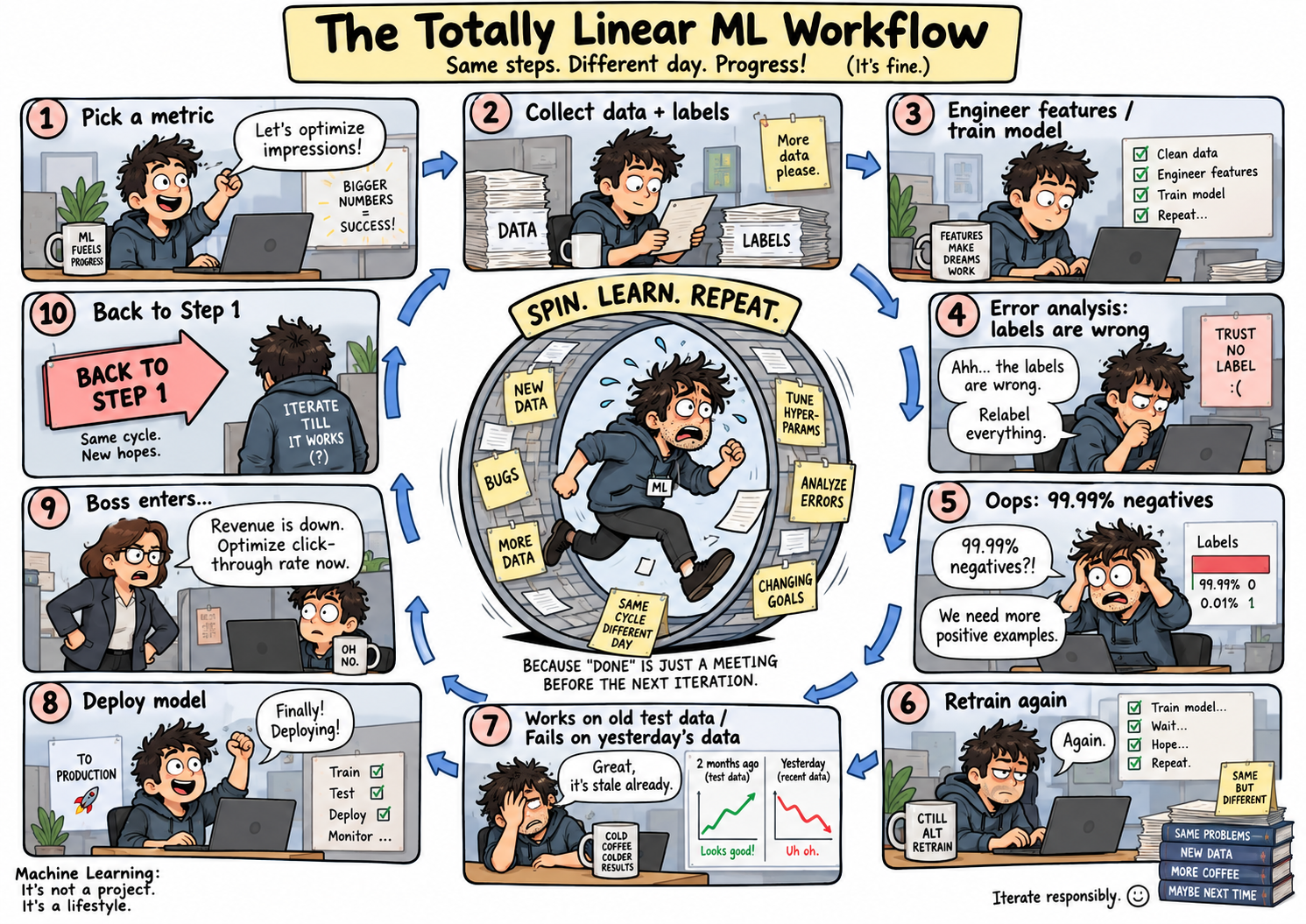
Here is a high level approach of the steps:

• Step 1. Project scoping

A project starts with scoping the project, laying out goals, objectives, and constraints. Stakeholders should be identified and involved. Resources should be estimated and allocated. Important: Here the ML project has to be scoped in the context of a business. Like Netflix recommendation systems impacts directly on streaming hours, and churn rate.

• Step 2. Data engineering

A vast majority of ML models today learn from data, so developing ML models starts with engineering data.

• Step 3. ML model development

With the initial set of training data, we’ll need to extract features and develop initial models leveraging these features. This is the stage that requires the most ML knowledge and is most often covered in ML courses.

• Step 4. Deployment

After a model is developed, it needs to be made accessible to users.

• Step 5. Monitoring and continual learning

Once in production, models need to be monitored for performance decay and maintained to be adaptive to changing environments and changing requirements

• Step 6. Business analysis

Model performance needs to be evaluated against business goals and analyzed to generate business insights.

Framing ML Problems

Let’s say imagine that you work for a bank that aims millenial customers and your boss heard that the next block bank is using Machine Learning for speeding up the customer requests of the users, and he tasks you to fix this.

We need to be clever and identify that customer service is a problem, not a Machine Learning problem. Since a Machine Learning problem, is defined by inputs, outputs, and an objective function that guides a learning process.

So our task is to figure out where is the bottleneck, and then let’s say that you found that every time a customer request comes, it takes time because it is transferred from human resources to inventory to customer service, then it goes to security.

So now this has become a classification problem that you can solve.The input is the customer request. The output is the department the request should go to. The objective function is to minimize the difference between the predicted department and the actual department.

Types of ML Tasks

The most general types of ML tasks are classification and regression.

Classification versus regression

Classification models classify inputs into different categories. For example, you want to classify each email to be either spam or not spam. Regression models output a continuous value. An example is a house prediction model that outputs the price of a given house.

Binary versus multiclass classification

Within classification problems, the fewer classes there are to classify, the simpler the problem is.

Examples of binary classification include classifying whether a comment is toxic, whether a lung scan shows signs of cancer, whether a transaction is fraudulent.

When there are more than two classes, the problem becomes multiclass classification.

When the number of classes is high, such as disease diagnosis where the number of diseases can go up to thousands or product classifications where the number of products can go up to tens of thousands, we say the classification task has high cardinality.

The first challenge is in data collection. In my experience, ML models typically need at least 100 examples for each class to learn to classify that class. So if you have 1,000 classes, you already need at least 100,000 examples.

Multiclass versus multilabel classification

In both binary and multiclass classification, each example belongs to exactly one class. When an example can belong to multiple classes, we have a multilabel classification problem. For example, when building a model to classify articles into four topics: tech, entertainment, finance, and politics, an article can be in both tech and finance.

Out of all task types, multilabel classification is usually the one that I’ve seen companies having the most problems with. Multilabel means that the number of classes an example can have varies from example to example.

Multiple ways to frame a problem

Changing the way you frame your problem might make your problem significantly harder or easier.

Example:

Let’s say that our task is to predict which application the user is going to open next on his phone, and we initially approach this as a classification problem. We start gathering the user’s demographic information, environment, time, location, and previous apps used. Let’s say that N is the number of apps that we want to recommend.

Classification

User + context
      ↓
    Model
      ↓
[App 0: .20, App 1: .02, App 2: .04, ...]
          one N-dimensional output

Initially, this seems like the correct approach. However, since we are considering the output to be a probability distribution over N applications, every time we want to consider a new application, we might need to retrain our model because the number of possible outputs changes.

On the other hand, if we approach this with a regression model, our features are the user’s environment, time, location, and also the app’s features. Our output in this case is going to be a value between zero and one representing how likely the user is to open that app.

Regression

User + context + App 0 features → Model → 0.03
User + context + App 1 features → Model → 0.06
User + context + App 2 features → Model → 0.25

In this framing, we are not going to need to retrain the model when we want to consider a new application. We simply need to use the new application’s features as a new input.

Objective Functions

To learn, an ML model needs an objective function to guide the learning process. An objective function is also called a loss function, because the objective of the learning process is usually to minimize (or optimize) the loss caused by wrong predictions. For supervised ML RMSE or cross entropy.

Decoupling objectives

Framing ML problems can be tricky when you want to minimize multiple objective functions. Imagine you’re building a system to rank items on users’ newsfeeds.

We start with three objectives:

• Filter out spam
• Filter out NSFW content
• Rank posts by engagement: how likely users will click on it

However you realize that engaging posts can lead to questionable ethical concerns, so you add a layer to protect:

• Filter out spam
• Filter out NSFW content
• Filter out misinformation
• Rank posts by quality
• Rank posts by engagement: how likely users will click on it

If a post is engaging but it’s of questionable quality, should that post rank high or low?

Essentially, you want to minimize quality_loss: the difference between each post’s predicted quality and its true quality. Similarly, to rank posts by engagement, you first need to predict the number of clicks each post will get.

One approach is to combine these two losses into one loss and train one model to minimize that loss:

loss = ɑ quality_loss + β engagement_loss

Mind Versus Data

Progress in the last decade shows that the success of an ML system depends largely on the data it was trained on. Instead of focusing on improving ML algorithms, most companies focus on managing and improving their data.

Mind might be disguised as inductive biases or intelligent architectural designs. Data might be grouped together with computation since more data tends to require more computation.

Chapter 3. Data Engineering Fundamentals

The rise of ML in recent years is tightly coupled with the rise of big data. Large data systems, even without ML, are complex.

If you look into the data stack for different tech companies, it might seem like each is doing its own thing.

Storing data is only interesting if you intend on retrieving that data later. To retrieve stored data, it’s important to know not only how it’s formatted but also how it’s structured.

Knowing how to collect, process, store, retrieve, and process an increasingly growing amount of data is essential to people who want to build ML systems in production.

Data Sources.

One source is user input data, data explicitly input by users. Another source is system-generated data. This one includes various types of logs and system outputs such as model predictions. They can record the results of different jobs, including large batch jobs for data processing and model training.

A problem with ML system logs is: it can be hard to know where to look because signals are lost in the noise, and also is how to store a rapidly growing number of logs

There are also internal databases, generated by various services and enterprise applications in a company (inventory, customer relationship, users)

Example: When user enters a search query in Amazon “frozen” before hitting the database a couple of ML models have to analyze the query and determine what is the customer refering to, either “frozen food” or “Disney cartoon” then lookup inventory database.

Finally another data source is third-party data.

• First-party data is the data that your company already collects about your users or customers.

• Second-party data is the data collected by another company on their own customers that they make available to you, though you’ll probably have to pay for it.

• Third-party data companies collect data on the public who aren’t their direct customers.

Data Formats

Since data is commonly collected from different sources we need to persist it and it’s important to think about how the data will be used in the future so that the format you use will make sense. Some questions like these may be helpful:

• How should we store multimodal data like image, text?

• Where should we store it so it’s cheaper and fast to retrieve?

• How to store complex models so that we can run them in different hardwares?

The process of converting a data structure or object state into a format that can be stored or transmitted and reconstructed later is data serialization

Row-Major Versus Column-Major Format

Overall, row-major formats are better when you have to do a lot of writes, whereas columnmajor ones are better when you have to do a lot of column-based reads.

Text Versus Binary Format

Binary files are more compact. Here’s a simple example to show how binary files can save space compared to text files. Consider that you want to store the number 1000000. If you store it in a text file, it’ll require 7 characters, and if each character is 1 byte, it’ll require 7 bytes. If you store it in a binary file as int32, it’ll take only 32 bits or 4 bytes.

AWS recommends using the Parquet format because “the Parquet format is up to 2x faster to unload and consumes up to 6x less storage in Amazon S3, compared to text formats.

Data Models

Data models describe how data is represented. Let’s think of cars and the attributes we may persist like make, model, color and price. And we could also represent a car by its owner license plate and history of registered address.

First one may be useful for people into buying a car whereas the second model is useful for police when they need to track down a vehicle.

Declarative ML

With models being increasingly commoditized, model development is often the easier part. The hard part lies in feature engineering, data processing, model evaluation, data shift detection, continual learning, and so on.

Structured Versus Unstructured Data

Because business requirements change over time, committing to a predefined data schema can become too restricting. Or you might have data from multiple data sources that are beyond your 18 control, and it’s impossible to make them follow the same schema.

This is where unstructured data becomes appealing. Unstructured data doesn’t adhere to a predefined data schema. It’s usually text but can also be numbers, dates, images, audio, etc. For example, a text file of logs generated by your ML model is unstructured data.

A repository for storing structured data is called a data warehouse. A repository for storing unstructured data is called a data lake. Data lakes are usually used to store raw data before processing. Data warehouses are used to store data that has been processed into formats ready to be used.

Modes of Dataflow (3 types)

• Data Passing Through Databases

For example, to pass data from process A to process B, process A can write that data into a database, and process B simply reads from that database. This mode, however, doesn’t always work because of two reasons.

First, it requires that both processes must be able to access the same database. This might be infeasible, especially if the two processes are run by two different companies.

Second, it requires both processes to access data from databases, and read/write from databases can be slow, making it unsuitable for applications with strict latency requirements

• Data Passing Through Services

One way to pass data between two processes is to send data directly through a network that connects these two processes. To pass data from process B to process A, process A first sends a request to process B that specifies the data A needs, and B returns the requested data through the same network. Because processes communicate through requests, we say that this is request-driven.

This mode of data passing is tightly coupled with the service-oriented architecture. A service is a process that can be accessed remotely, e.g., through a network. In this example, B is exposed to A as a service that A can send requests to. For B to be able to request data from A, A will also need to be exposed to B as a service.

For example, a service might be run by a stock exchange that keeps track of the current stock prices. Another service might be run by an investment firm that requests the current stock prices and uses them to predict future stock prices.

Structuring an application as separate services gives you a microservice architecture.

Let’s use Lyft as example (extremely simplified):

• Driver management service Predicts how many drivers will be available in the next minute in a given area.

• Ride management service Predicts how many rides will be requested in the next minute in a given area.

• Price optimization service Predicts the optimal price for each ride. The price for a ride should be low enough for riders to be willing to pay, yet high enough for drivers to be willing to drive and for the company to make a profit.

Implementations of a REST architecture are said to be RESTful. Even though many people think of REST as HTTP, REST doesn’t exactly mean HTTP because HTTP is just an implementation of REST. (We may think of REST as architectural style)

• Data Passing Through Real-Time Transport

To understand the motivation for real-time transports, let’s go back to the preceding example of the ride-sharing app with three simple services: driver management, ride management, and price optimization.

Now, imagine that the driver management service also needs to know the number of rides from the ride management service to know how many drivers to mobilize. It also wants to know the predicted prices from the price optimization service to use them as incentives for potential drivers (e.g., if you get on the road now you can get a 2x surge charge).

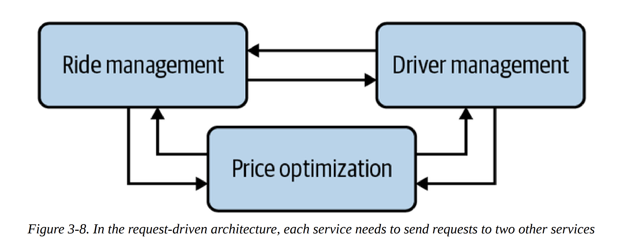
Similarly, the ride management service might also want data from the driver management and price optimization services. If we pass data through services as discussed in the previous section, each of these services needs to send requests to the other two services. With only three services, data passing is already getting complicated.

Request-driven data passing is synchronous: the target service has to listen to the request for the request to go through. If the price optimization service requests data from the driver management service and the driver management service is down, the price optimization service will keep resending the request until it times out.

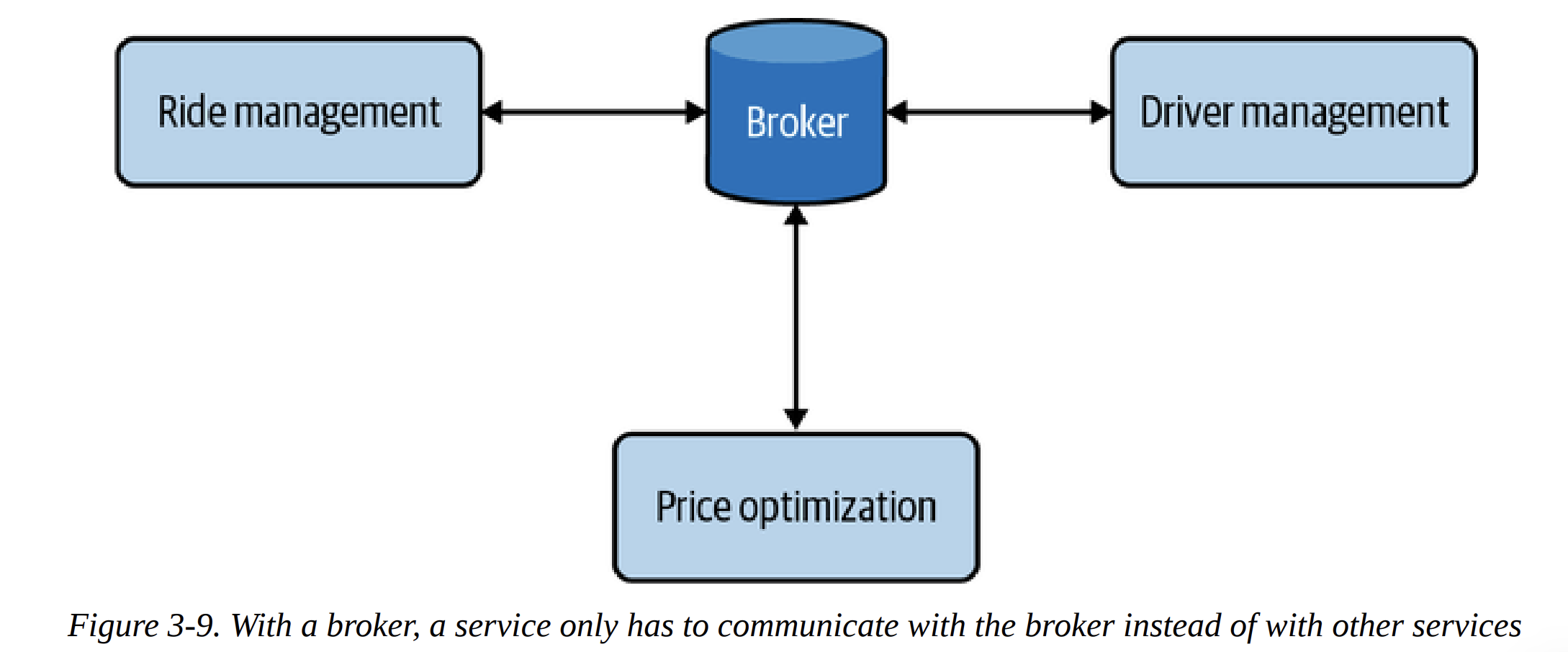
What if there’s a broker that coordinates data passing among services? Instead of having services request data directly from each other and creating a web of complex interservice data passing, each service only has to communicate with the broker

Whichever service wants data from the driver management service can check that broker for the most recent predicted number of drivers. Similarly, whenever the price optimization service makes a prediction about the surge charge for the next minute, this prediction is broadcast to the broker.

Request-driven architecture works well for systems that rely more on logic than on data. Eventdriven architecture works better for systems that are data-heavy.

The two most common types of real-time transports are pubsub, which is short for publishsubscribe, and message queue.

Batch Processing Versus Stream Processing

Once your data arrives in data storage engines like databases, data lakes, or data warehouses, it becomes historical data. This is opposed to streaming data (data that is still streaming in). Historical data is often processed in batch jobs—jobs that are kicked off periodically. For example, once a day. (batch processing)

When you have data in real-time transports like Apache Kafka and Amazon Kinesis, we say that you have streaming data. Stream processing refers to doing computation on streaming data. Computation on streaming data can also be kicked off periodically, but the periods are usually much shorter than the periods for batch jobs.

Because batch processing happens much less frequently than stream processing, in ML, batch processing is usually used to compute features that change less often, such as drivers’ ratings (if a driver has had hundreds of rides, their rating is less likely to change significantly).

Batch features—features extracted through batch processing—are also known as static features.

Stream processing is used to compute features that change quickly, such as how many drivers are available right now, how many rides have been requested in the last minute, how many rides will be finished in the next two minutes, the median price of the last 10 rides in this area.

Streaming features—features extracted through stream processing are also known as dynamic features.

For many problems, you need not only batch features or streaming features, but both. You need infrastructure that allows you to process streaming data as well as batch data and join them together to feed into your ML models.

For ML systems that leverage streaming features, the streaming computation is rarely simple. The number of stream features used in an application such as fraud detection and credit scoring can be in the hundreds, if not thousands. The stream feature extraction logic can require complex queries with join and aggregation along different dimensions.

Stream processing is more difficult because the data amount is unbounded and the data comes in at variable rates and speeds. It’s easier to make a stream processor do batch processing than to make a batch processor do stream processing.

Chapter 4. Training Data (Sampling, labeling, class imbalance, data augmentation)

Many ML practitioners and courses lean more towards the “fun” part of modeling the data, when the real work happens before that phase, in the preprocessing, cleasing of the data. This chapter goes over how to prepare those datasets correctly so we can start the “modeling” phase properly and avoid asking ourselves “what are we feeding our model with?”

This chapter starts with different sampling techniques to select data for training. We’ll then address common challenges in creating training data, including the label multiplicity problem, the lack of labels problem, the class imbalance problem, and techniques in data augmentation to address the lack of data problem.

We use the term “training data” instead of “training dataset” because “dataset” denotes a set that is finite and stationary. Data in production is neither finite nor stationary. Like other steps in building ML systems, creating training data is an iterative process.

Sampling

In this section, we’ll focus on sampling methods for creating training data, but these sampling methods can also be used for other steps in an ML project lifecycle.

In many cases, sampling is necessary. One case is when you don’t have access to all possible data in the real world, the data that you use to train your model is a subset of real-world data. Another case is when it’s infeasible to process all the data that you have access to.

Sampling is helpful as it allows you to accomplish a task faster and cheaper

For example, when considering a new model, you might want to do a quick experiment with a small subset of your data to see if the new model is promising first before training this new model on all your data

Understanding different sampling methods and how they are being used in our workflow can, first, help us avoid potential sampling biases, and second, help us choose the methods that improve the efficiency of the data we sample.

There are two families of sampling: nonprobability sampling and random sampling.

Nonprobability Sampling

Nonprobability sampling is when the selection of data isn’t based on any probability criteria. Here are some of the criteria for nonprobability sampling:

• Convenience sampling
• Snowball sampling
• Judgement sampling
• Quota sampling

The samples selected by nonprobability criteria are not representative of the real-world data and therefore are riddled with selection biases.

One example of these cases is language modeling. Language models are often trained not with data that is representative of all possible texts but with data that can be easily collected—Wikipedia, Common Crawl, Reddit.

Another example: IMDB reviews and Amazon reviews are biased toward users who are willing to leave reviews online, and not necessarily representative of people who don’t have access to the internet or people who aren’t willing to put reviews online.

Nonprobability sampling can be a quick and easy way to gather your initial data to get your project off the ground. However, for reliable models, you might want to use probability-based sampling, which we will cover next.

Simple Random Sampling

In the simplest form of random sampling, you give all samples in the population equal probabilities of being selected. For example, you randomly select 10% of the population, giving all members of this population an equal 10% chance of being selected. The drawback is that rare categories of data might not appear in your selection.

Stratified Sampling

To avoid the drawback of simple random sampling, you can first divide your population into the groups that you care about and sample from each group separately. For example, to sample 1% of data that has two classes, A and B, you can sample 1% of class A and 1% of class B. This way, no matter how rare class A or B is, you’ll ensure that samples from it will be included in the selection.

One drawback of this sampling method is that it isn’t always possible, such as when it’s impossible to divide all samples into groups. This is especially challenging when one sample might belong to multiple groups, as in the case of multilabel tasks. For instance, a sample can be both class A and class B.

Weighted Sampling

In weighted sampling, each sample is given a weight, which determines the probability of it being selected. For example, if you have three samples, A, B, and C, and want them to be selected with the probabilities of 50%, 30%, and 20% respectively, you can give them the weights 0.5, 0.3, and 0.2.

This method allows you to leverage domain expertise. For example, if you know that a certain subpopulation of data, such as more recent data, is more valuable to your model and want it to have a higher chance of being selected, you can give it a higher weight.

Reservoir Sampling

Reservoir sampling is a fascinating algorithm that is especially useful when you have to deal with streaming data, which is usually what you have in production.

Imagine you have an incoming stream of tweets and you want to sample a certain number. You want to ensure that:

• Every tweet has an equal probability of being selected.

• You can stop the algorithm at any time and the tweets are sampled with the correct probability.

Main idea: Keep exactly k items in memory from a stream of unknown size, while making sure every item seen so far has the same probability of being in the sample.

import random

def reservoir_sampling(stream, k):
  reservoir = []

  for n, item in enumerate(stream, start=1):

      # First k items: just store them
      if n <= k:
          reservoir.append(item)

      else:
          # Generate random integer from 1 to n
          i = random.randint(1, n)

          # If i falls inside the reservoir positions
          if i <= k:
              reservoir[i - 1] = item

  return reservoir

Importance Sampling

Example with LLM help:

Suppose you care about distribution P, but can only sample from Q:

| x | P(x) target | Q(x) sampled | Weight P/Q |
| - | ----------: | -----------: | ---------: |
| 1 |        0.10 |         0.50 |   0.2× |
| 2 |        0.30 |         0.30 |     1× |
| 3 |        0.60 |         0.20 |     3× |

`Q` gives us too many 1s, so each `1` counts less (`0.2×`). It gives us the right amount of `2s`, so they count normally (`1×`). It gives us too few 3s, so each `3` counts more (`3×`).

Sample from what you can access (`Q`), then reweight it to represent what you actually care about (`P`).

Labeling

Despite the promise of unsupervised ML, most ML models in production today are supervised, which means that they need labeled data to learn from. The performance of an ML model still depends heavily on the quality and quantity of the labeled data it’s trained on.

In a talk to my students, Andrej Karpathy, director of AI at Tesla, shared an anecdote about how when he decided to have an in-house labeling team, his recruiter asked how long he’d need this team for. He responded: “How long do we need an engineering team for?”

Hand Labels

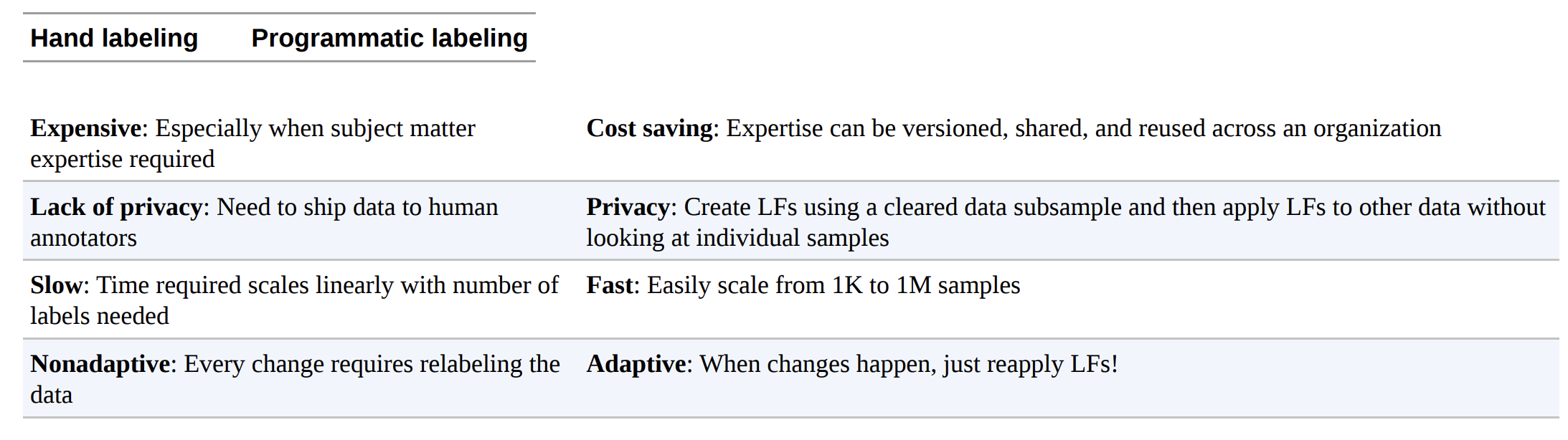
Anyone who has ever had to work with data in production has probably felt this at a visceral level: acquiring hand labels for your data is difficult for many, many reasons. First, hand-labeling data can be expensive, especially if subject matter expertise is required. To classify whether a comment is spam, you might be able to find 20 annotators on a crowdsourcing platform and train them in 15 minutes to label your data. However, if you want to label chest X-rays, you’d need to find board-certified radiologists, whose time is limited and expensive.

Second, hand labeling poses a threat to data privacy. Third, hand labeling is slow. For example, accurate transcription of speech utterance at the phonetic level can take 400 times longer than the utterance duration.

Slow labeling leads to slow iteration speed and makes your model less adaptive to changing environments and requirements. If the task changes or data changes, you’ll have to wait for your data to be relabeled before updating your model.

Label multiplicity

Often, to obtain enough labeled data, companies have to use data from multiple sources and rely on multiple annotators who have different levels of expertise. These different data sources and annotators also have different levels of accuracy.

What to do when there are multiple conflicting labels for a data instance. Consider this simple task of entity recognition. You give three annotators the following sample and ask them to annotate all entities they can find:

Darth Sidious, known simply as the Emperor, was a Dark Lord of the Sith who reigned over the galaxy as Galactic Emperor of the First Galactic Empire.

Perhaps 3, 4, 6? To minimize the disagreement among annotators, it’s important to first have a clear problem definition. For example, in the preceding entity recognition task, some disagreements could have been eliminated if we clarify that in case of multiple possible entities, pick the entity that comprises the longest substring. This means “Galactic Emperor of the First Galactic Empire” instead of “Galactic Emperor” and “First Galactic Empire”.

Data lineage

Indiscriminately using data from multiple sources, generated with different annotators, without examining their quality can cause your model to fail mysteriously. Your ML engineers are confident that more data will improve the model performance, so you spend a lot of money to hire annotators to label another million data samples.

However, the model performance actually decreases after being trained on the new data. The reason is that the new million samples were crowdsourced to annotators who labeled data with much less accuracy than the original data.

It’s good practice to keep track of the origin of each of your data samples as well as its labels, a technique known as data lineage. Data lineage helps you both flag potential biases in your data and debug your models. For example, if your model fails mostly on the recently acquired data samples, you might want to look into how the new data was acquired.

On more than one occasion, we’ve discovered that the problem wasn’t with our model, but because of the unusually high number of wrong labels in the data that we’d acquired recently.

Natural Labels

Hand-labeling isn’t the only source for labels. You might be lucky enough to work on tasks with natural ground truth labels. Tasks with natural labels are tasks where the model’s predictions can be automatically evaluated or partially evaluated by the system.

Example: Google Maps knows how long the trip actually took, and thus can evaluate the accuracy of the predicted time of arrival.

The canonical example of tasks with natural labels is recommender systems. The goal of a recommender system is to recommend to users items relevant to them. Whether a user clicks on the recommended item or not can be seen as the feedback for that recommendation. A recommendation that gets clicked on can be presumed to be good (i.e., the label is POSITIVE) and a recommendation that doesn’t get clicked on after a period of time, say 10 minutes, can be presumed to be bad (i.e., the label is NEGATIVE).

Natural labels that are inferred from user behaviors like clicks and ratings are also known as behavioral labels.

Another example, if you’re building a machine translation system like Google Translate, you can have the option for the community to submit alternative translations for bad translations these alternative translations can be used to train the next iteration of your models (though you might want to review these suggested translations first)

Like button and other reactions to each newsfeed item, Facebook is able to collect feedback on their ranking algorithm.

Tasks with natural labels are fairly common in the industry. In a survey of 86 companies in my network, I found that 63% of them work with tasks with natural labels, this means that companies find it easier and cheaper to first start on tasks that have natural labels.

In the previous example, a recommendation that doesn’t get clicked on after a period of time can be presumed to be bad. This is called an implicit label, as this negative label is presumed from the lack of a positive label. It’s different from explicit labels where users explicitly demonstrate their feedback on a recommendation by giving it a low rating or downvoting it.

Feedback loop length

For tasks with natural ground truth labels, the time it takes from when a prediction is served until when the feedback on it is provided is the feedback loop length. Tasks with short feedback loops are tasks where labels are generally available within minutes.

If you work with longer content types like blog posts or articles or YouTube videos, the feedback loop can be hours.

DIFFERENT TYPES OF USER FEEDBACK

For example, consider an ecommerce application similar to what Amazon has. Types of feedback a user on this application can provide might include clicking on a product recommendation, adding a product to cart, buying a product, rating, leaving a review, and returning a previously bought product.

Clicking on a product happens much faster and more frequently (and therefore incurs a higher volume) than purchasing a product. However, buying a product is a much stronger signal on whether a user likes that product compared to just clicking on it.

Labels with long feedback loops are helpful for reporting a model’s performance on quarterly or yearly business reports. However, they are not very helpful if you want to detect issues with your models as soon as possible.

Feedback Loop Time Window

Choosing the right window length requires thorough consideration, as it involves the speed and accuracy tradeoff. A short window length means that you can capture labels faster, which allows you to use these labels to detect issues with your model and address those issues as soon as possible. However, a short window length also means that you might prematurely label a recommendation as bad before it’s clicked on.

Handling the Lack of Labels

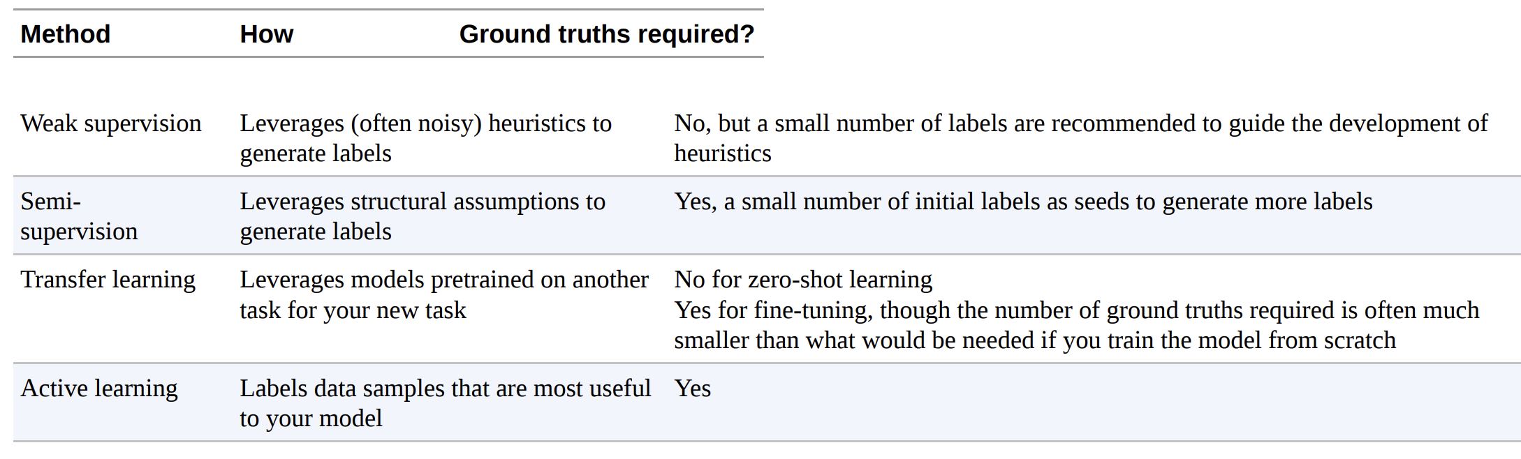
Because of the challenges in acquiring sufficient high-quality labels, many techniques have been developed to address the problems that result. In this section, we will cover four of them: weak supervision, semisupervision, transfer learning, and active learning.

1. Weak supervision

This technique relies on heuristics, which can be developed with subject matter expertise, to label data. For example, a doctor might use the following heuristics to decide whether a patient’s case should be prioritized as emergent:

“If the nurse’s note mentions a serious condition like pneumonia, the patient’s case should be given priority consideration.”

def labeling_function(note):
  if "pneumonia" in note:
    return "EMERGENT"

LFs can encode many different types of heuristics. Here are some of them:

• Keyword heuristic
• Regular expressions
• Database lookup
• The outputs of other models

Because LFs encode heuristics, and heuristics are noisy, labels produced by LFs are noisy. Multiple LFs might apply to the same data examples, and they might give conflicting labels. One function might think a nurse’s note is EMERGENT but another function might think it’s not.

With LFs, subject matter expertise can be versioned, reused, and shared. Expertise owned by one team can be encoded and used by another team. If your data changes or your requirements change, you can just reapply LFs to your data samples. The approach of using LFs to generate labels for your data is also known as programmatic labeling.

Weak supervision is a simple but powerful paradigm. However, it’s not perfect. In some cases, the labels obtained by weak supervision might be too noisy to be useful. But even in these cases, weak supervision can be a good way to get you started when you want to explore the effectiveness of ML without wanting to invest too much in hand labeling up front.

1. Semi-supervision

If weak supervision leverages heuristics to obtain noisy labels, semi-supervision leverages structural assumptions to generate new labels based on a small set of initial labels. Unlike weak supervision, semisupervision requires an initial set of labels.

A classic semi-supervision method is self-training. You start by training a model on your existing set of labeled data and use this model to make predictions for unlabeled samples. Assuming that predictions with high raw probability scores are correct, you add the labels predicted with high probability to your training set and train a new model on this expanded training set.

Another semi-supervision method assumes that data samples that share similar characteristics share the same labels.

Semi-supervision is the most useful when the number of training labels is limited. One thing to consider when doing semi-supervision with limited data is how much of this limited data should be used to evaluate multiple candidate models and select the best one. If you use a small amount, the best performing model on this small evaluation set might be the one that overfits the most to this set.

On the other hand, if you use a large amount of data for evaluation, the performance boost gained by selecting the best model based on this evaluation set might be less than the boost gained by adding the evaluation set to the limited training set. Many companies overcome this trade-off by using a reasonably large evaluation set to select the best model, then continuing training the champion model on the evaluation set.

So the practical idea is: Use enough labeled data to reliably choose the model, then once you’ve chosen the champion, let that model learn from those labeled examples too.

1. Transfer learning

Transfer learning refers to the family of methods where a model developed for a task is reused as the starting point for a model on a second task.

First, the base model is trained for a base task. The base task is usually a task that has cheap and abundant training data.

Language modeling is a great candidate because it doesn’t require labeled data. Language models can be trained on any body of text—books, Wikipedia articles, chat histories—and the task is: given a sequence of tokens, predict the next token. When given the sequence “I bought NVIDIA shares because I believe in the importance of,” a language model might output “hardware” or “GPU” as the next token.

Transfer learning is especially appealing for tasks that don’t have a lot of labeled data. Even for tasks that have a lot of labeled data, using a pretrained model as the starting point can often boost the performance significantly compared to training from scratch.

Transfer learning has gained a lot of interest in recent years for the right reasons. It has enabled many applications that were previously impossible due to the lack of training samples. A nontrivial portion of ML models in production today are the results of transfer learning, including object detection models that leverage models pretrained on ImageNet and text classification models that leverage pretrained language models such as BERT or GPT-3.

Active learning

Active learning is a method for improving the efficiency of data labels. The hope here is that ML models can achieve greater accuracy with fewer training labels if they can choose which data samples to learn from. Active learning is sometimes called query learning.

Instead of randomly labeling data samples, you label the samples that are most helpful to your models according to some metrics or heuristics. You label the examples that your model is the least certain about, hoping that they will help your model learn the decision boundary better.

Another common heuristic is based on disagreement among multiple candidate models. This method is called query-by-committee, an example of an ensemble method. Each model can make one vote for which samples to label next, and it might vote based on how uncertain it is about the prediction. You then label the samples that the committee disagrees on the most.

Class Imbalance

Class imbalance typically refers to a problem in classification tasks where there is a substantial difference in the number of samples in each class of the training data. For example, in a training dataset for the task of detecting lung cancer from X-ray images, 99.99% of the X-rays might be of normal lungs, and only 0.01% might contain cancerous cells.

Class imbalance can also happen with regression tasks where the labels are continuous. Consider the task of estimating health-care bills. When predicting hospital bills, it might be more important to predict accurately the bills at the 95th percentile than the median bills. A 100% difference in a $250 bill is acceptable (actual $500, predicted $250), but a 100% difference on a $10k bill is not (actual $20k, predicted $10k). Therefore, we might have to train the model to be better at predicting 95th percentile bills, even if it reduces the overall metrics.

Challenges of Class Imbalance

ML, especially deep learning, works well in situations when the data distribution is more balanced, and usually not so well when the classes are heavily imbalanced.

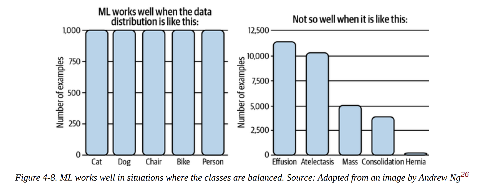
The first reason is that class imbalance often means there’s insufficient signal for your model to learn to detect the minority classes. In the case where there is a small number of instances in the minority class, the problem becomes a few-shot learning problem where your model only gets to see the minority class a few times before having to make a decision on it. In the case where there is no instance of the rare classes in your training set, your model might assume these rare classes don’t exist.

The second reason is that class imbalance makes it easier for your model to get stuck in a nonoptimal solution by exploiting a simple heuristic instead of learning anything useful about the underlying pattern of the data. Consider the preceding lung cancer detection example. If your model learns to always output the majority class, its accuracy is already 99.99%. This heuristic can be very hard for gradient descent algorithms to beat because a small amount of randomness added to this heuristic might lead to worse accuracy.

The third reason is that class imbalance leads to asymmetric costs of error—the cost of a wrong prediction on a sample of the rare class might be much higher than a wrong prediction on a sample of the majority class. For example, misclassification on an X-ray with cancerous cells is much more dangerous than misclassification on an X-ray of a normal lung.

If your loss function isn’t configured to address this asymmetry, your model will treat all samples the same way. As a result, you might obtain a model that performs equally well on both majority and minority classes, while you much prefer a model that performs less well on the majority class but much better on the minority one.

The classical example of tasks with class imbalance is fraud detection. Most credit card transactions are not fraudulent. As of 2018, 6.8¢ for every $100 in cardholder spending is fraudulent.

Another cause for class imbalance, though less common, is due to labeling errors. Annotators might have read the instructions wrong or followed the wrong instructions (thinking there are only two classes, POSITIVE and NEGATIVE, while there are actually three), or simply made errors.

Handling Class Imbalance

There have been many techniques suggested to mitigate the effect of class imbalance. However, as neural networks have grown to be much larger and much deeper, with more learning capacity, some might argue that you shouldn’t try to “fix” class imbalance if that’s how the data looks in the real world. A good model should learn to model that imbalance. However, developing a model good enough for that can be challenging, so we still have to rely on special training techniques.

In this section, we will cover three approaches to handling class imbalance:

• choosing the right metrics for your problem;

• data-level methods, which means changing the data distribution to make it less imbalanced; and

• algorithm-level methods, which means changing your learning method to make it more robust to class imbalance.

Using the right evaluation metrics

The most important thing to do when facing a task with class imbalance is to choose the appropriate evaluation metrics. Wrong metrics will give you the wrong ideas of how your models are doing and, subsequently, won’t be able to help you develop or choose models good enough for your task.

• Confusion matrix, F1, recall, MSE, RMSE, MAE, R2.

Data-level methods: Resampling

Data-level methods modify the distribution of the training data to reduce the level of imbalance to make it easier for the model to learn. A common family of techniques is resampling. Resampling includes oversampling, adding more instances from the minority classes, and undersampling, removing instances of the majority classes.

When you resample your training data, never evaluate your model on resampled data, since it will cause your model to overfit to that resampled distribution.

Undersampling runs the risk of losing important data from removing data. Oversampling runs the risk of overfitting on training data, especially if the added copies of the minority class are replicas of existing data. Many sophisticated sampling techniques have been developed to mitigate these risks.

One such technique is two-phase learning. You first train your model on the resampled data. This resampled data can be achieved by randomly undersampling large classes until each class has only N instances. You then fine-tune your model on the original data.

Another technique is dynamic sampling: oversample the low-performing classes and undersample the highperforming classes during the training process.

Algorithm-level methods

If data-level methods mitigate the challenge of class imbalance by altering the distribution of your training data, algorithm-level methods keep the training data distribution intact but alter the algorithm to make it more robust to class imbalance.

Because the loss function (or the cost function) guides the learning process, many algorithm-level methods involve adjustment to the loss function. The key idea is that if there are two instances, x and x , and the loss resulting from making the wrong prediction on x is higher than x , the model will prioritize making the correct prediction on x over making the correct prediction on x . By giving the training instances we care about higher weight, we can make the model focus more on learning these instances.

There are many ways to modify this cost function.

• Cost-sensitive learning

• Class-balanced loss

• Focal loss

Data Augmentation

Data augmentation is a family of techniques that are used to increase the amount of training data. Traditionally, these techniques are used for tasks that have limited training data, such as in medical imaging. However, in the last few years, they have shown to be useful even when we have a lot of data.

In this section, we will cover three main types of data augmentation: simple label-preserving transformations; perturbation, which is a term for “adding noises”; and data synthesis. In each type, we’ll go over examples for both computer vision and NLP.

• Simple Label-Preserving Transformations

• Perturbation

• Data Synthesis

One of the most notable perturbation examples is BERT, where the model chooses 15% of all tokens in each sequence at random and chooses to replace 10% of the chosen tokens with random words. For example, given the sentence “My dog is hairy,” and the model randomly replacing “hairy” with “apple,” the sentence becomes “My dog is apple.” So 1.5% of all tokens might result in nonsensical meaning. Their ablation studies show that a small fraction of random replacement gives their model a small performance boost

Data synthesis example: In NLP, templates can be a cheap way to bootstrap your model. One team I worked with used templates to bootstrap training data for their conversational AI (chatbot). A template might look like: “Find me a [CUISINE] restaurant within [NUMBER] miles of [LOCATION]” (see Table 4-10). With lists of all possible cuisines, reasonable numbers (you would probably never want to search for restaurants beyond 1,000 miles), and locations (home, office, landmarks, exact addresses) for each city, you can generate thousands of training queries from a template.

Summary

Training data still forms the foundation of modern ML algorithms. No matter how clever your algorithms might be, if your training data is bad, your algorithms won’t be able to perform well. It’s worth it to invest time and effort to curate and create training data that will enable your algorithms to learn something meaningful.

Most ML algorithms in use today are supervised ML algorithms, so obtaining labels is an integral part of creating training data. Many tasks, such as delivery time estimation or recommender systems, have natural labels. Natural labels are usually delayed, and the time it takes from when a prediction is served until when the feedback on it is provided is the feedback loop length. Tasks with natural labels are fairly common in the industry, which might mean that companies prefer to start on tasks that have natural labels over tasks without natural labels.

For tasks that don’t have natural labels, companies tend to rely on human annotators to annotate their data. However, hand labeling comes with many drawbacks. For example, hand labels can be expensive and slow. To combat the lack of hand labels, we discussed alternatives including weak supervision, semi-supervision, transfer learning, and active learning.

ML algorithms work well in situations when the data distribution is more balanced, and not so well when the classes are heavily imbalanced. Unfortunately, problems with class imbalance are the norm in the real world. In the following section, we discussed why class imbalance made it hard for ML algorithms to learn. We also discussed different techniques to handle class imbalance, from choosing the right metrics to resampling data to modifying the loss function to encourage the model to pay attention to certain samples.