domi lizarraga
I read Natural Language Processing in Action: Understanding, analyzing, and generating text with Python by Hobson Lane, Cole Howard & Hannes Max Hapke on September 10, 2026
Review
Currently reading. Notes in progress.
Notes
This book is divided in 3 parts and it assumes you already know Python. It does contain code snippets and exercises we can run in our machines.
Part I is a brief introduction to classic NLP, like doing each step at the time, going from English sentence, tokenize them, then vectorize and lastly apply topic vectors in order to compress those numerical representations. This is useful for semantic search to chatbots.
Part II starts using some Neural Networks and more modern algorithm like backpropagation and libraries like Word2Vec the type of NN (neural network are presented in the book are CNN and RNN).
Part III is meant for building a real project using most modern NLP.
Chapter 1. Packets of thought (NLP overview)
In this chapter the book goes over what really is NLP, difference of “natural language” vs “programming language” and incrementally we add more tools to build our chatbot.
Natural language is used for communicate each other, it doesn’t need an interpreter/compiler, it doesn’t process math operations like a Programming language does. However we need to process Natural language in a way that computer can understand so that it act on those statements or even reply to them, we need to make those statements into data (numbers).
A natural language processing system is often referred to as a pipeline because it usually involves several stages, where input is natural languge and a processed output flows out.
The size of the actual natural language content currently online must exceed 100 billion gigabytes.
Natural languages can’t be directly translated into a precise set of mathematical operations, but they do contain information and instructions that can be extracted.
The math.
Processing natural language to extract useful information can be difficult. It requires tedious statistical bookkeeping, but that’s what machines are for.
Once you extract structured numerical data, vectors, from natural language, you can take advantage of all the tools of mathematics and machine learning.
We use the same linear algebra tricks as the projection of 3D objects onto a 2D computer screen, allowing computers to interpret and store the “meaning” of statements rather than just word or character counts. Semantic analysis, along with statistics, can help resolve the ambiguity of natural language.
Here is another challenge for computer to understand Natural language and it’s “decoding” which is having the current context when a phrase is said. Like when someone says: “Good morning.” What makes a morining good? What about noons and afternoons?
This degree of compression is still out of reach for machines.
Language through a computer’s “eyes”
When you type “Good Morn’n Rosa,” a computer sees only “01000111 01101111 01101111 …”. How can you program a chatbot to respond to this binary stream intelligently?
For some mechanical pattern matching we can use either lock language statements, such as “01-02-03” or Regular expressions. Amazon Echo, Google Home, and similarly complex and useful assistants use this kind of language to encode the logic for most of their user interaction.
Regular expressions are indeed used mostly for search, for sequence matching. Example: grep
This pattern matching chatbot is an example of a tightly controlled chatbot.
The first regex recognizes simple greetings such as hi, hello, and hey, optionally followed by a name.
import re
r = "(hi|hello|hey)[ ]*([a-z]*)"

# IGNORECASE igonores uppercase/lowercase differences
re.match(r, "Hello Rosa", flags=re.IGNORECASE)
# match='Hello Rosa'

re.match(r, "hi ho, hi ho, it's off to work ...", flags=re.IGNORECASE)
# match='hi ho'

re.match(r, "hey, what's up", flags=re.IGNORECASE)
# match='hey'
A version with a more flexible greeting:
r = r"[^a-z]*([y]o|[h']?ello|ok|hey|(good[ ])?(morn[gin']{0,3}|"\"
re_greeting = re.compile(r, flags=re.IGNORECASE)
re_greeting.match("Hello Rosa")
re_greeting.match("Good morning Rosa")
re_greeting.match("Good Morn'n Rosa")
re_greeting.match("yo Rosa")
re_greeting.match("Good evening Rosa Parks").groups()

# ('Good evening', 'Good ', 'evening', 'Rosa')
A modern chatbot can learn from reading (processing) a bunch of English text. Also these two versiones don’t allow typos or last name from the user since we are only pattern matching first name characters.
Because of the limitations of computational resources, early NLP researchers had to use their human brains’ computational power to design and hand-tune complex logical rules to extract information from a natural language string. This is called a pattern based approach to NLP.
The core NLP building blocks like stemmers and tokenizers as well as sophisticated end-to-end NLP dialog engines (chatbots) like ELIZA were built this way, from regular expressions and pattern matching
Another way.
Is there a statistical or machine learning approach that might work in place of the pattern-based approach?
When we use character sequence matches to measure distance between natural language phrases, we’ll often get it wrong. Phrases with similar meaning, like “good” and “okay,” can often have different character sequences and large distances when we count up character-by-character.
And sequences with completely different meanings, like “bad” and “bar,” might be too close to one other when we use metrics designed to measure distances between numerical sequences. Metrics like Jaccard, Levenshtein, and Euclidean vector distance can sometimes add enough “fuzziness” to prevent a chatbot from stumbling over minor spelling errors or typos. But these metrics fail to capture the essence of the relationship between two strings of characters when they are dissimilar.
Distance metrics designed for numerical sequences and vectors are useful for a few NLP applications, like spelling correctors and recognizing proper nouns. So we use these distance metrics when they make sense.
But for NLP applications where we are more interested in the meaning of the natural language than its spelling, there are better approaches. We use vector representations of natural language words and text and some distance metrics for those vectors for these NLP applications.
Using statistics, machine learning and more data. We nned to use vector for storing the words based on frequency and meaning, see how the “bag of words” can be represented by removing stop-words, rare-words:
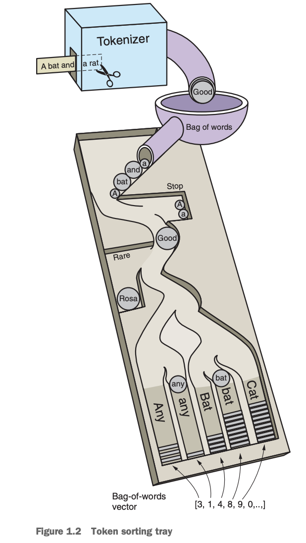
Those bins and the numbers they contain for each word are represented as long vectors containing a lot of zeros and a few ones or twos scattered around wherever the word for that bin occurred.
Sentence: "A bat and a rat"

Embedding (illustrative): [0.2323, -0.4210, 0.8732]

Word frequencies:
{
  "a": 2,
  "bat": 1,
  "and": 1,
  "rat": 1
}
(many bins, one for each possible word) aren’t very useful for language processing. But they are good enough for some industry-changing tools like spam filters
One statistical question that is asked of bag-of-words vector sequences is “What is the combination of words most likely to follow a particular bag of words?” Or, even better, if a user enters a sequence of words, “What is the closest bag of words in our database to a bag-of-words vector provided by the user?” This is a search query.
Theinput words are the words you might type into a search box, and the closest bag-of-words vector corresponds to the document or web page you were looking for.
A brief overflight of hyperspace.
When we project these vectors onto each other to determine the distance between pairs of vectors, this will be a reasonable estimate of the similarity in their meaning rather than merely their statistical word usage
This vector distance metric is called cosine distance metric.
We can even project (“embed” is the more precise term) these vectors in a 2D plane to have a “look” at them in plots and diagrams to see if our human brains can find patterns.
We can then teach a computer to recognize and act on these patterns in ways that reflect the underlying meaning of the words that produced those vectors.
Here is another aproach to represent high dimension vectors called a bit vector language model, or the sum of “one-hot encoded” vectors.
Sentence: "A bat and a rat" (lowercased before counting)
Our vocabulary also includes "dog", which is absent here.

Vocabulary:       a   bat  and  rat  dog
                  ↓    ↓    ↓    ↓    ↓
One-hot vector for each word occurrence:
  "a"           [ 1,   0,   0,   0,   0 ]
  "bat"         [ 0,   1,   0,   0,   0 ]
  "and"         [ 0,   0,   1,   0,   0 ]
  "a"           [ 1,   0,   0,   0,   0 ]
  "rat"         [ 0,   0,   0,   1,   0 ]
                ─────────────────────────
Sum (counts):   [ 2,   1,   1,   1,   0 ]  → 5 dimensions
                  │
                  │ Change every positive count to 1
                  ↓
Bit vector:     [ 1,   1,   1,   1,   0 ]  → 5 dimensions
                  ↑                   ↑
               present              absent

Each bit answers: "Does this word appear in the sentence?"
Summing one-hot vectors for DISTINCT words also gives this bit vector.
We lose repetition counts, not dimensions: still one position per word
in the vocabulary.
- Count vectors measure occurrences.
- Binary vectors record presence.
- Rating vectors describe chosen properties.
- Learned embeddings encode patterns learned from data.
Word order and grammar.
When we have short sentences like “Good morning Rosa” order doesn’t matter, but when dealing with longer strings, the order is key.
A chatbot natural language pipeline.
Most chatbots contain elements of these stages:
1 Parse—Extract features, structured numerical data, from natural language text.
2 Analyze—Generate and combine features by scoring text for sentiment, grammaticality, and semantics.
3 Generate—Compose possible responses using templates, search, or language models.
4 Execute—Plan statements based on conversation history and objectives, and select the next response.
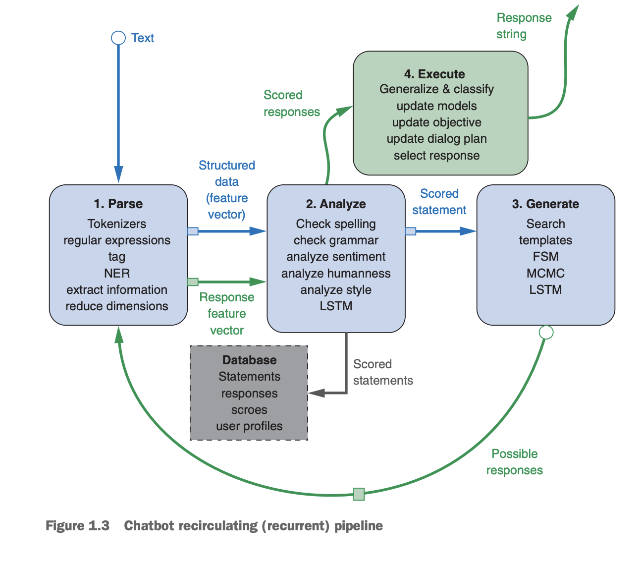
One processing element in figure 1.3 that isn’t typically employed in search, forecasting, or question answering systems is natural language generation.
Processing in depth.
Chapter 2. Build your vocabulary (word tokenization)
This chapter will help you split a document, any string, into discrete tokens of meaning. Dealing with nonstandard punctuation. Compressing your token vocabulary with stemming and lemmatization. Building a vector representation.
Retrieving tokens from a document will require some string manipulation beyond just the
str.split().
Once you’ve identified the tokens in a document that you’d like to include in your vocabulary, you’ll return to the regular expression toolbox to try to combine words with similar meaning in a process called stemming.
Then you’ll assemble a vector representation of your documents called a bag of words then try to use this vector to see if it can help you improve upon the greeting recognizer
In this chapter, we show you straightforward algorithms for separating a string into words. You’ll also extract pairs, triplets, quadruplets, and even quintuplets of tokens. These are called
n-grams
Using n-grams enables your machine to know about “ice cream” as well as the “ice” and “cream” that comprise it.
In natural language processing, composing a numerical vector from text is a particularly “lossy” feature extraction process. Nonetheless the bag-of-words (BOW) vectors retain enough of the information content of the text to produce useful and interesting machine learning models.
Feature extraction can rarely retain all the information content of the input data in any machine learning pipeline. That’s part of the art of NLP, learning when your tokenizer needs to be adjusted to extract more or different information from your text for your particular application.
In NLP, composing a numerical vector from text is a particularly “lossy” feature extraction process. Nonetheless the bag-of-words (BOW) vectors retain enough of the information content of the text to produce useful and interesting machine learning models.
Building your vocabulary with a tokenizer
In NLP, tokenization is a particular kind of document segmentation. Segmentation breaks up text into smaller chunks or segments, with more focused information content. Segmentation can include breaking a document into paragraphs, paragraphs into sentences, sentences into phrases, or phrases into tokens (usually words) and punctuation
Tokenization is the first step in an NLP pipeline, so it can have a big impact on the rest of your pipeline. A tokenizer breaks unstructured data, natural language text, into chunks of information that can be counted as discrete elements.
.split()this built-in Python method already does a decent job tokenizing a simple sentence. Its only “mistake” was on the last word, where it included the sentence-ending punctuation with the token “26.”
One hot vectors are nice representation of words and tabular representation of documents is that no information is lost. As long as you keep track of which words are indicated by which column, you can reconstruct the original document from this table of one-hot vectors.
import pandas as pd

pd.DataFrame(onehot_vectors, columns=vocab)
   26.  Jefferson  Monticello  Thomas  age  at  began  building  of  the
0    0          0           0       1    0   0      0         0   0    0
1    0          1           0       0    0   0      0         0   0    0
2    0          0           0       0    0   0      1         0   0    0
3    0          0           0       0    0   0      0         1   0    0
4    0          0           1       0    0   0      0         0   0    0
5    0          0           0       0    0   1      0         0   0    0
6    0          0           0       0    0   0      0         0   0    1
7    0          0           0       0    1   0      0         0   0    0
8    0          0           0       0    0   0      0         0   1    0
9    1          0           0       0    0   0      0         0   0    0
However, mathematically is not practical. It grows pretty quickly. And what you really want to do is compress the meaning of a document down to its essence. You’d like to compress your document down to a single vector rather than a big table.
What if you split your documents into much shorter chunks of meaning, say sentences. And what if you assumed that most of the meaning of a sentence can be gleaned from just the words themselves. Let’s assume you can ignore the order and grammar of the words, and jumble them all up together into a “bag,” one bag for each sentence or short document. That turns out to be a reasonable assumption. Even for documents several pages long, a bag-of-words vector is still useful for summarizing the essence of a document.
You can use this new bag-of-words vector approach to compress the information content for each document into a data structure that’s easier to work with.
This is also called a word frequency vector, because it only counts the frequency of words, not their order.
Dot product
The dot product is also called the inner product because the “inner” dimension of the two vectors (the number of elements in each vector) or matrices (the rows of the first matrix and the columns of the second matrix) must be the same.
The dot product is also called the scalar product because it produces a single scalar value as its output. This helps distinguish it from the cross product, which produces a vector as its output.
python = np.array([0.9, 0.1])
javascript = np.array([0.8, 0.1])
pizza = np.array([0.1, 0.9])

print(python @ javascript) # 0.73
print(python @ pizza) # 0.18

Python · JavaScript = 0.73
Python · pizza      = 0.18

# This tells us that Pythin and JS vectors are more aligned than Python and pizza.
Constraint: For a dot product, the inner dimensions must match. For two vectors, this simply means they must have the same length.
Measuring bag-of-words overlap
If we can measure the bag of words overlap for two vectors, we can get a good estimate of how similar they are in the words they use. And this is a good estimate of how similar they are in meaning.
a = "I like machine learning"
b = "I like deep learning"

unique_words = ["I", "like", "machine", "deep", "learning"]

A = [1, 1, 1, 0, 1]
B = [1, 1, 0, 1, 1]

A · B = 3

# because the sentences share three words: I, like, and learning.
As you can imagine, tokenizers can easily become complex. In one case, you might want to split based on periods, but only if the period isn’t followed by a number, in order to avoid splitting decimals. In another case, you might not want to split after a period that is part of “smiley” emoticon symbol, such as in a Twitter message.
The important thing is that you’ve turned a sentence of natural language words into a sequence of numbers, or vectors. Now you can have the computer read and do math on the vectors just like any other vector or list of numbers. This allows your vectors to be input into any natural language processing pipeline that requires this kind of vector
Python NLP libraries:
- spaCy—Accurate , flexible, fast, Python
- Stanford CoreNLP—More accurate, less flexible, fast, depends on Java 8
- NLTK—Standard used by many NLP contests and comparisons, popular, Python
An even better tokenizer is the Treebank Word Tokenizer from the NLTK package. It incorporates a variety of common rules for English word tokenization. ` TreebankWordTokenizer()`
Extending your vocabulary with n-grams
Why bother with n-grams? As you saw earlier, when a sequence of tokens is vectorized into a bag-of-words vector, it loses a lot of the meaning inherent in the order of those words. By extending your concept of a token to include multiword tokens, n-grams, your NLP pipeline can retain much of the meaning inherent in the order of words in your statements.
For example, the meaning-inverting word “not” will remain attached to its neighboring words, where it belongs. Without n-gram tokenization, it would be free floating. Its meaning would be associated with the entire sentence or document rather than its neighboring words. The 2-gram “was not” retains much more of the meaning of the individual words “not” and “was” than those 1-grams alone in a bag-of-words vector.
In the next chapter, we show you how to recognize which of these n-grams contain the most information relative to the others, which you can use to reduce the number of tokens (n-grams) your NLP pipeline has to keep track of. Otherwise it would have to store and maintain a list of every single word sequence it came across. This prioritization of n-grams will help it recognize “Thomas Jefferson” and “ice cream,” without paying particular attention to “Thomas Smith” or “ice shattered.”
The later stages of your NLP pipeline will only have access to whatever tokens your tokenizer generates. So you need to let those later stages know that “Thomas” wasn’t about “Isaiah Thomas” or the “Thomas & Friends” cartoon. n-grams are one of the ways to maintain context information as data passes through your pipeline.
# 1-gram VS 2-gram VS 3-gram

"""Thomas Jefferson began building Monticello at the age of 26."""

['Thomas',
'Jefferson',
'began',
'building',
'Monticello',
'at',
'the',
'age',
'of',
'26']

[('Thomas', 'Jefferson'),
('Jefferson', 'began'),
('began', 'building'),
('building', 'Monticello'),
('Monticello', 'at'),
('at', 'the'),
('the', 'age'),
('age', 'of'),
('of', '26')]

[('Thomas', 'Jefferson', 'began'),
('Jefferson', 'began', 'building'),
('began', 'building', 'Monticello'),
('building', 'Monticello', 'at'),
('Monticello', 'at', 'the'),
('at', 'the', 'age'),
('the', 'age', 'of'),
('age', 'of', '26')]
If tokens or n-grams are extremely rare, they don’t carry any correlation with other words that you can use to help identify topics or themes that connect documents or classes of documents. So rare n-grams won’t be helpful for classification problems.
If your feature vector dimensionality exceeds the length of all your documents, your feature extraction step is counterproductive. It’ll be virtually impossible to avoid overfitting a machine learning model to your vectors; your vectors have more dimensions than there are documents in your corpus.
Now consider the opposite problem. Consider the 2-gram “at the” in the previous phrase. That’s probably not a rare combination of words. In fact it might be so common, spread among most of your documents, that it loses its utility for discriminating between the meanings of your documents.
For example, if a token or n-gram occurs in more than 25% of all the documents in your corpus, you usually ignore it.
These filters are as useful for n-grams as they are for individual tokens. In fact, they’re even more useful.
Stop words.
Stop words include: a, an, the, this, and, or, of, on.
Historically, stop words have been excluded from NLP pipelines in order to reduce the computational effort to extract information from a text. Even though the words themselves carry little information, the stop words can provide important relational information as part of an n-gram.
Consider these two examples: Mark reported to the CEO. Suzanne reported as the CEO to the board.
If you remove the stop words from the 4-grams, both examples would be reduced to “reported CEO”, and you would lack the information about the professional hierarchy.
Unfortunately, retaining the stop words within your pipeline creates another problem: it increases the length of the n-grams required to make use of these connections formed by the otherwise meaningless stop words. This issue forces us to retain at least 4-grams if you want to avoid the ambiguity of the human resources example.
A typical stop word list has only 100 or so frequent and unimportant words listed in it.
For 100,000-D bag-ofwords vectors, you usually must have 100,000 labeled examples, and sometimes even more than that, to train a supervised machine learning pipeline without overfitting. In some situations, cutting your vocabulary size by half can be worth the loss of information content.
IMPORTANT! The best way to find out what works is to try several different approaches, and see which approach gives you the best performance for the objectives of your NLP project.
By generalizing your model to work with text that has odd capitalization, case normalization can reduce overfitting for your machine learning pipeline.
Stemming
For example, the words housing and houses share the same stem, house. Stemming removes suffixes from words in an attempt to combine words with similar meanings together under their common stem.
In machine learning this is referred to as dimension reduction.
So, as long as your application doesn’t require your machine to distinguish between “house” and “houses,” this stem will reduce your programming or dataset size by half or even more.
Stemming is important for keyword search or information retrieval. It allows you to search for “developing houses in Portland” and get web pages or documents that use both the word “house” and “houses” and even the word “housing,” because these words are all stemmed to the “hous” token.
This broadening of your search results would be a big improvement in the “recall” score for how well your search engine is doing its job at returning all the relevant documents.
But stemming could greatly reduce the “precision” score for your search engine, because it might return many more irrelevant documents along with the relevant ones. In some applications this “false-positive rate”
Lemmatization
It reduces the number of words you have to respond to, the dimensionality of your language model. Using it can make your model more general, but it can also make your model less precise, because it will treat all spelling variations of a given root word the same. For example “chat,” “chatter,” “chatty,” “chatting,” and perhaps even “chatbot” would all be treated the same in an NLP pipeline.
Lemmatization is a potentially more accurate way to normalize a word than stemming or case normalization because it takes into account a word’s meaning. A lemmatizer uses a knowledge base of word synonyms and word endings to ensure that only words that mean similar things are consolidated into a single token.
Consider the word better. Stemmers would strip the “er” ending from “better” and return the stem “bett” or “bet.” However, this would lump the word “better” with words like “betting,” “bets,” and “Bet’s,” rather than more similar words like “betterment,” “best,” or even “good” and “goods.”
So lemmatizers are better than stemmers for most applications. Stemmers are only really used in large-scale information retrieval applications (keyword search). And if you really want the dimension reduction and recall improvement of a stemmer in your information retrieval pipeline, you should probably also use a lemmatizer right before the stemmer. Because the lemma of a word is a valid English word, stemmers work well on the output of a lemmatizer.
Use cases
When should you use a lemmatizer or a stemmer? Stemmers are generally faster to compute and require less-complex code and datasets. But stemmers will make more errors and stem a far greater number of words, reducing the information content or meaning of your text much more than a lemmatizer would.
Both stemmers and lemmatizers will reduce your vocabulary size and increase the ambiguity of the text. But lemmatizers do a better job retaining as much of the information content as possible based on how the word was used within the text and its intended meaning.
If your application involves search, stemming and lemmatization will improve the recall of your searches by associating more documents with the same query words. However, stemming, lemmatization, and even case folding will significantly reduce the precision and accuracy of your search results.
If your application involves search, stemming and lemmatization will improve the recall of your searches by associating more documents with the same query words. However, stemming, lemmatization, and even case folding will significantly reduce the precision and accuracy of your search results. These vocabulary compression approaches will cause an information retrieval system (search engine) to return many documents not relevant to the words’ original meanings.
IMPORTANT Bottom line, try to avoid stemming and lemmatization unless you have a limited amount of text that contains usages and capitalizations of the words you are interested in. And with the explosion of NLP datasets, this is rarely the case for English documents, unless your documents use a lot of jargon or are from a very small subfield of science, technology, or literature.
Sentiment
Whether you use raw single-word tokens, n-grams, stems, or lemmas in your NLP pipeline, each of those tokens contains some information. An important part of this information is the word’s sentiment—the overall feeling or emotion that the word invokes.
Companies like to know what users think of their products. So they often will provide some way for you to give feedback. A star rating on Amazon or Rotten Tomatoes is one way to get quantitative data about how people feel about products they’ve purchased. But a more natural way is to use natural language comments. Giving your user a blank slate (an empty text box) to fill up with comments about your product can produce more detailed feedback.
An NLP pipeline can process a large quantity of user feedback quickly and objectively, with less chance for bias. And an NLP pipeline can output a numerical rating of the positivity or negativity or any other emotional quality of the text.
There are two approaches to sentiment analysis: A rule-based algorithm composed by a human A machine learning model learned from data by a machine
The first approach to sentiment analysis uses human-designed rules, sometimes called heuristics, to measure sentiment. A common rule-based approach to sentiment analysis is to find keywords in the text and map each one to numerical scores or weights in a dictionary or “mapping”.
The second approach, machine learning, relies on a labeled set of statements or documents to train a machine learning model to create those rules. A machine learning sentiment model is trained to process input text and output a numerical value for the sentiment you are trying to measure, like positivity or spamminess or trolliness. For the machine learning approach, you need a lot of data, text labeled with the “right” sentiment score.
Chapter 3. Math with words (TF-IDF vectors)
This chapter covers counting words and term frequencies to analyze meaning, predicting word occurrence probabilities, vector representation of words, finding relevant documents from a corpus using inverse document frequencies and estimating the similarity with cosine and BM25.
Having collected and counted words (tokens), and bucketed them into stems or lemmas, it’s time to do something interesting with them. Detecting words is useful for simple tasks, like getting statistics about word usage or doing keyword search. But you’d like to know which words are more important to a particular document and across the corpus as a whole.
Then you can use that “importance” value to find relevant documents in a corpus based on keyword importance within each document.
The next step in your adventure is to turn the words of chapter 2 into continuous numbers rather than just integers representing word counts or binary “bit vectors” that detect the presence or absence of particular words.
Your goal is to find numerical representation of words that somehow capture the importance or information content of the words they represent. You’ll have to wait until chapter 4 to see how to turn this information content into numbers that represent the meaning of words.
We’ll look at three increasingly powerful ways to represent words and their importance in a document:
- Bags of words—Vectors of word counts or frequencies
- Bags of n-grams—Counts of word pairs (bigrams), triplets (trigrams)
- TF-IDF vectors—Word scores that better represent their importance
IMPORTANT TF-IDF stands for term frequency times inverse document frequency. Term frequencies are the counts of each word in a document, which you learned about in previous chapters. Inverse document frequency means that you’ll divide each of those word counts by the number of documents in which the word occurs.
Each of these techniques can be applied separately or as part of an NLP pipeline. These are all statistical models in that they are frequency based.
Bag of words
In the previous chapter, you created your first vector space model of a text. You used one-hot encoding of each word and then combined all those vectors with a binary OR (or clipped sum) to create a vector representation of a text.
You then looked at an even more useful vector representation that counts the number of occurrences, or frequency, of each word in the given text.
As a first approximation, you assume that the more times a word occurs, the more meaning it must contribute to that document.
from nltk.tokenize import TreebankWordTokenizer
from collections import Counter

sentence = """The faster Harry got to the store, the faster Harry,
... the faster, would get home."""
tokenizer = TreebankWordTokenizer()
tokens = tokenizer.tokenize(sentence.lower())
tokens
['the',
'faster',
'harry',
'got',
'to',
'the',
'store',
',',
'the',
'faster',
'harry',
',',
'the',
'faster',
',',
'would',
'get',
'home',
'-']

bag_of_words = Counter(token
bag_of_words

Counter({'the': 4,
  'faster': 3,
  'harry': 2,
  'got': 1,
  'to': 1,
  'store': 1,
  ',': 3,
  'would': 1,
  'get': 1,
  'home': 1,
  '.': 1})
For short documents like this one, the unordered bag of words still contains a lot of information about the original intent of the sentence. And the information in a bag of words is sufficient to do some powerful things such as detect spam, compute sentiment (positivity, happiness, and so on), and even detect subtle intent, like sarcasm.
Let’s pause for a second and look a little deeper at normalized term frequency, a phrase (and calculation) we use often throughout this book.
bag_of_words.most_common(4)
[('the', 4), (',', 3), ('faster', 3), ('harry', 2)]

times_harry_appears = bag_of_words['harry']
num_unique_words = len(bag_of_words)

tf = times_harry_appears / num_unique_words
round(tf, 4)
0.1818
Let’s say you find the word “dog” 3 times in document A and 100 times in document B. Clearly “dog” is way more important to document B. But wait. Let’s say you find out document A is a 30-word email to a veterinarian and document B is War & Peace (approx 580,000 words!).
TF(“dog,” documentA) = 3/30 = .1
TF(“dog,” documentB) = 100/580000 = .00017
Now you have something you can see that describes “something” about the two documents and their relationship to the word “dog” and each other. So instead of raw word counts to describe your documents in a corpus, you can use normalized term frequencies. Similarly you could calculate each word and get the relative importance to the document of that term. Your protagonist, Harry, and his need for speed are clearly central to the story of this document.
Vectorizing
You’ve transformed your text into numbers on a basic level. But you’ve still just stored them in a dictionary, so you’ve taken one step out of the text-based world and into the realm of mathematics. Next you’ll go ahead and jump in all the way. Instead of describing a document in terms of a frequency dictionary, you’ll make a vector of those word counts.
document_vector = []
doc_length = len(tokens)
for key, value in kite_counts.most_common():
    document_vector.append(value / doc_length)
document_vector
[0.07207207207207207,
0.06756756756756757,
0.036036036036036036,
...,
0.0045045045045045045]
Having one vector for one document isn’t enough. You can grab a couple more documents and make vectors for each of them as well. But the values within each vector need to be relative to something consistent across all the vectors. If you’re going to do math on them, they need to represent a position in a common space, relative to something consistent.
Your vectors need to have the same origin and share the same scale, or “units,” on each of their dimensions.
The first step in this process is to normalize the counts by calculating normalized term frequency instead of raw count in the document (as you did in the last section); the second step is to make all the vectors of standard length or dimension.
This collections of words in your vocabulary is often called a lexicon, which is the same concept referenced in earlier chapters, just in terms of your special corpus.
from collections import Counter

# docs is 3 docuemnts

docs = [
    "The faster Harry got to the store, the faster and faster Harry would get home.",
    "Harry is hairy and faster than Jill.",
    "Jill is not as hairy as Harry."
]

tokenized_docs = [
    doc.lower()
       .replace(",", "")
       .replace(".", "")
       .split()
    for doc in docs
]

vocab = sorted(set(
    token
    for doc in tokenized_docs
    for token in doc
))

['and', 'as', 'faster', 'get', 'got', 'hairy', 'harry',
 'home', 'is', 'jill', 'not', 'store', 'than', 'the',
 'to', 'would']


# Now convert each document into a word-count vector using the same vocabulary:

def vectorize(tokens, vocab):
    counts = Counter(tokens)

    return [counts[word] for word in vocab]

doc_vectors = [
    vectorize(tokens, vocab)
    for tokens in tokenized_docs
]

for vector in doc_vectors:
    print(vector)

Document 1 → [1, 0, 3, 1, 1, 0, 2, 1, 0, 0, 0, 1, 0, 3, 1, 1]
Document 2 → [1, 0, 1, 0, 0, 1, 1, 0, 1, 1, 0, 0, 1, 0, 0, 0]
Document 3 → [0, 2, 0, 0, 0, 1, 1, 0, 1, 1, 1, 0, 0, 0, 0, 0]

# The important idea is that every position always represents the same word:

              and  as  faster  get  got  hairy  harry  ...
Document 1 →   1    0     3     1    1     0      2    ...
Document 2 →   1    0     1     0    0     1      1    ...
Document 3 →   0    2     0     0    0     1      1    ...

# So we now have three vectors, one for each document, all living in the same vector space.
Vector spaces
A vector space is the set of all possible vectors with the same number of dimensions. A vector with 2 values lives in 2D, 3 values in 3D, and an NLP document with thousands of features can live in a space with thousands of dimensions.
2D vector space

y
↑
|        • (3,2)
|       /
|      /
|     /
|____/____________→ x
(0,0)

vector = [3, 2]
In NLP, each dimension can represent a feature or vocabulary term, and each document becomes a point/vector in that shared space.
For a natural language document vector space, the dimensionality of your vector space is the count of the number of distinct words that appear in the entire corpus. For TF (and TF-IDF to come), sometimes we call this dimensionality capital letter “K.” This number of distinct words is also the vocabulary size of your corpus, so in an academic paper it’ll usually be called “ V .” You can then describe each document within this K-dimensional vector space by a K-dimensional vector. K = 18 in your threedocument corpus about Harry and Jill.
Euclidean distance cares about both direction and magnitude, while cosine similarity mainly cares about direction. In NLP, direction is often more useful because documents of different lengths can still use words in very similar proportions.
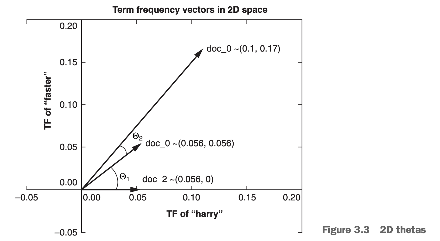
For NLP document vectors that have a cosine similarity close to 1, you know that the documents are using similar words in similar proportion. A cosine similarity of 0 represents two vectors that share no components. They are orthogonal, perpendicular in all dimensions.
Zipf’s Law (predicting word occurrence)
Specifically, inverse proportionality refers to a situation where an item in a ranked list will appear with a frequency tied explicitly to its rank in the list. The first item in the ranked list will appear twice as often as the second, and three times as often as the third, for example.
Topic modeling
Inverse document frequency, or IDF, is your window through Zipf in topic analysis. Let’s take your term frequency counter from earlier and expand on it. You can count tokens and bin them up two ways: per document and across the entire corpus. You’re going to be counting just by document.
A good way to think of a term’s inverse document frequency is this: How strange is it that this token is in this document? If a term appears in one document a lot of times, but occurs rarely in the rest of the corpus, one could assume it’s important to that document specifically. Your first step toward topic analysis!
from collections import Counter
import math

# Suppose we have two documents:

docs = {
    "intro": """
    A kite is traditionally a tethered aircraft.
    Kites have been used in China for centuries.
    """,

    "history": """
    The history of kites goes back thousands of years.
    Kites were used for communication and military purposes.
    """
}

# Normalize and tokenize them:

tokens = {
    name: text.lower()
              .replace(".", "")
              .replace(",", "")
              .split()
    for name, text in docs.items()
}

counts = {
    name: Counter(doc_tokens)
    for name, doc_tokens in tokens.items()
}


## 1. Term Frequency (TF)

# Term Frequency measures how common a word is inside one document:

def tf(term, doc_name):
    return counts[doc_name][term] / len(tokens[doc_name])

print(tf("kite", "intro"))
print(tf("kite", "history"))


# A word may have a high TF simply because it appears many times in a document.


## 2. Document Frequency

# Now ask a different question:

# > In how many documents does this word appear?

def document_frequency(term):
    return sum(
        term in doc_tokens
        for doc_tokens in tokens.values()
    )

print(document_frequency("kite"))
print(document_frequency("china"))

# If a word appears in every document, it is less useful for distinguishing them.

# If it appears in only one document, it may carry more information.


## 3. Inverse Document Frequency (IDF)

# IDF gives more weight to rare words:

def idf(term):
    num_docs = len(tokens)
    docs_with_term = document_frequency(term)

    return math.log(num_docs / docs_with_term)

print(idf("kite"))
print(idf("china"))

# A common word gets a lower IDF.

# A rarer word gets a higher IDF.


## 4. TF-IDF

def tfidf(term, doc_name):
    return tf(term, doc_name) * idf(term)

terms = ["kite", "china", "and"]

for term in terms:
    print(
        term,
        "intro:",
        round(tfidf(term, "intro"), 4),
        "history:",
        round(tfidf(term, "history"), 4),
    )
TF measures how important a word is inside one document, while IDF reduces the importance of words that appear across many documents. TF-IDF combines both.
Return of Zipf
Zipf’s Law suggests that raw frequency differences can become disproportionately large, so TF-IDF uses a logarithm to compress those differences. (We need to scale it)
#Suppose we have a corpus of: 1,000,000 documents

# "cat" appears in 1 document
# "dog" appears in 10 documents
# "the" appears in 900,000 documents

# Without logarithmic scaling:
num_docs = 1_000_000
cat_idf_raw = num_docs / 1
dog_idf_raw = num_docs / 10
the_idf_raw = num_docs / 900_000
print(cat_idf_raw)  # 1000000
print(dog_idf_raw)  # 100000
print(the_idf_raw)  # 1.111...


# Without log:

# cat → 1,000,000
# dog →   100,000
# the →         1.11

# The differences are enormous.
# Now apply log10():

import math
cat_idf_log = math.log10(num_docs / 1)
dog_idf_log = math.log10(num_docs / 10)
the_idf_log = math.log10(num_docs / 900_000)
print(cat_idf_log)  # 6.0
print(dog_idf_log)  # 5.0
print(the_idf_log)  # ~0.046


# With log:

# cat → 6.000
# dog → 5.000
# the → 0.046

So:
WITHOUT LOG                WITH LOG

cat  █████████████████     cat  ██████
dog  ██                    dog  █████
the  ·                     the  ·

# without log → "cat" is 10x more important than "dog"
# with log    → "cat" is only slightly more important than "dog"
Relevance ranking
# Start with a shared vocabulary:


vocabulary = [the, harry, store, faster, is, jill]

# Represent a document using raw word counts:

doc_0 = [3, 2, 1, 3, 0, 0]


# Each position corresponds to the same vocabulary term:


                #  the   harry   store   faster   is   jill

# word count        3      2       1       3      0     0


# Raw counts are not ideal because common words may dominate even if they are not very informative.

# So replace each count with a TF-IDF weight:


#                  the   harry   store   faster   is   jill

# word count        3      2       1       3      0     0
#                    ↓      ↓       ↓       ↓
# TF-IDF           .02    .18     .15      .22     0     0


# TF-IDF combines two ideas:


# TF
# How common is this word
# inside THIS document?

# IDF
# How unusual or informative is this word
# across ALL documents?


# common everywhere
#         ↓
# low IDF
#         ↓
# low TF-IDF weight

# rare across corpus
# but important here
#         ↓
# high IDF
#         ↓
# higher TF-IDF weight


# Now each document becomes a TF-IDF vector:


doc_0 = [0.02, 0.18, 0.15, 0.22, 0, 0]
doc_1 = [...]
doc_2 = [...]


# Then treat the search query as another document:


query = "How long does it take to get to the store?"


# Convert it into a TF-IDF vector using the same vocabulary:


query_vec = [...]


# Finally, compare the query vector against every document vector using cosine similarity:


# query_vec
#     │
#     ├── cosine similarity → doc_0 = 0.5235
#     ├── cosine similarity → doc_1 = 0.0000
#     └── cosine similarity → doc_2 = 0.0000


# Higher cosine similarity means the vectors point in a more similar direction:


# higher cosine similarity
#         ↓
# more similar TF-IDF patterns
#         ↓
# more relevant document

# QUERY:
# How long does it take TO GET TO THE STORE?

# DOC 0:
# The faster Harry GOT TO THE STORE,
# the faster and faster Harry would GET HOME.

#  Similar words:
# to
# get
# the
# store
TF-IDF improves raw word-count vectors by giving more weight to terms that are important in a document but relatively rare across the corpus. Cosine similarity can then rank documents by how closely their weighted term distributions match the query.
Keyword search is only one tool in your NLP pipeline. need to take one additional step to turn your simple search index (TF-IDF) into a chatbot. You need to store your training data in pairs of questions (or statements) and appropriate responses. Then you can use TF-IDF to search for a question (or statement) most like the user input text. Instead of returning the most similar statement in your database, you return the response associated with that statement.
TF-IDF in practice and alternatives
Instead of implementing TF-IDF manually,
scikit-learnprovidesTfidfVectorizer, which can tokenize the corpus, build the vocabulary, compute TF-IDF weights, and return the result as a sparse matrix.
from sklearn.feature_extraction.text import TfidfVectorizer

vectorizer = TfidfVectorizer()
tfidf_matrix = vectorizer.fit_transform(docs)
Each row represents a document, each column represents a term in the vocabulary, and each cell contains that term’s TF-IDF weight.
Because most documents use only a small fraction of the total vocabulary, the matrix is usually sparse:
                 harry   faster   jill   store   ...
document_0        .48      .64      0      .21
document_1        .37      .37     .49      0
document_2        .22       0      .38      0
TF-IDF is a strong lexical baseline: it matches documents based on weighted word overlap, but more advanced approaches can go beyond exact keyword matching and capture semantic relationships.
One such alternative to using straight TF-IDF cosine distance to rank query results is Okapi BM25, or its most recent variant, BM25F.
You can optimize your pipeline by choosing the weighting scheme that gives your users the most relevant results. But if your corpus isn’t too large, you might consider forging ahead with us into even more useful and accurate representations of the meaning of words and documents.
In subsequent chapters, we show you how to implement a semantic search engine that finds documents that “mean” something similar to the words in your query rather than just documents that use those exact words from your query. Semantic search is much better than anything TF-IDF weighting and stemming and lemmatization can ever hope to achieve.
The only reason Google and Bing and other web search engines don’t use the semantic search approach is that their corpus is too large. Semantic word and topic vectors don’t scale to billions of documents, but millions of documents are no problem.
BM25 improves on basic TF-IDF ranking by combining IDF with term-frequency saturation and document-length normalization. Repeating a term helps, but with diminishing returns, and matching a term in a short focused document is often more valuable than matching it in a very long one.
TF-IDF: How important is this term?
BM25: How important is this term, how often does it appear, and how long is the document?
Chapter 4. Finding meaning in word counts (semantic analysis)
We will cover: analyzing semantics (meaning) to create topic vectors, semantic search between topic vectors, scalable semantic analysis, using semantic components and navigating high-dimensional vector spaces.
This is the first time we talk about a machine being able to understand the “meaning” of words.
The TF-IDF vectors (term frequency–inverse document frequency vectors) from chapter 3 helped you estimate the importance of words in a chunk of text. You used TF-IDF vectors and matrices to tell you how important each word is to the overall meaning of a bit of text in a document collection.
Past NLP experimenters found an algorithm for revealing the meaning of word combinations and computing vectors to represent this meaning. It’s called latent semantic analysis (LSA). And when you use this tool, not only can you represent the meaning of words as vectors, but you can use them to represent the meaning of entire documents.
In this chapter, you’ll learn about these semantic or topic vectors. You’re going to use your weighted frequency scores from TF-IDF vectors to compute the topic “scores” that make up the dimensions of your topic vector. These topic vectors will help you do a lot of interesting things. They make it possible to search for documents based on their meaning—semantic search.
Most of the time, semantic search returns search results that are much better than keyword search (TFIDF search). Sometimes semantic search returns documents that are exactly what the user is searching for, even when they can’t think of the right words to put in the query.
And you can use these semantic vectors to identify the words and n-grams that best represent the subject (topic) of a statement, document, or corpus (collection of documents).
Example:
Sentence A:
"The car is very fast"
Sentence B:
"The automobile is really quick"
Sentence C:
"I like cooking pasta"
A purely word-based representation may not see A and B as very similar because:
car ≠ automobile
fast ≠ quick
very ≠ really
A semantic representation tries to capture relationships such as:
car        ≈ automobile
fast       ≈ quick
Suppose the semantic dimensions roughly represent:
[transportation, speed, food]
Then the sentences could be represented as:
A = [0.80, 0.70, 0.10]
B = [0.75, 0.72, 0.08]
C = [0.05, 0.10, 0.90]
We can compare them with cosine similarity:
import numpy as np

def cosine_similarity(a, b):
    return np.dot(a, b) / (
        np.linalg.norm(a) * np.linalg.norm(b)
    )

a = np.array([0.80, 0.70, 0.10])
b = np.array([0.75, 0.72, 0.08])
c = np.array([0.05, 0.10, 0.90])

print(cosine_similarity(a, b))
print(cosine_similarity(a, c))
Conceptually:
A vs B → very high similarity
A vs C → low similarity
So:
"The car is very fast"
        ≈
"The automobile is really quick"

similarity → very high
while:
"The car is very fast"
        ≠
"I like cooking pasta"

similarity → low
In this chapter, you’re learning how to build an NLP pipeline that can figure out this kind of synonymy, all on its own. Your pipeline might even be able to find the similarity in meaning of the phrase “figure it out” and the word “compute.” Machines can only “compute” meaning, not “figure out” meaning.
From word counts to topic scores
You know how to count the frequency of words. And you know how to score the importance of words in a TF-IDF vector or matrix. But that’s not enough. You want to score the meanings, the topics, that words are used for.
TF-IDF vectors count the exact spellings of terms in a document. So texts that restate the same meaning will have completely different TF-IDF vector representations if they spell things differently or use different words. This messes up search engines and document similarity comparisons that rely on counts of tokens.
In chapter 2, you normalized word endings so that words that differed only in their last few characters were collected together under a single token. You used normalization approaches such as stemming and lemmatization to create small collections of words with similar spellings, and often similar meanings, and then you processed these new tokens instead of the original words.
This lemmatization approach kept similarly spelled words together in your analysis, but not necessarily words with similar meanings. And it definitely failed to pair up most synonyms. Synonyms usually differ in more ways than just the word endings that lemmatization and stemming deal with.
Even worse, lemmatization and stemming sometimes erroneously lump together antonyms, words with opposite meaning.
The end result is that two chunks of text that talk about the same thing but use different words will not be “close” to each other in your lemmatized TF-IDF vector space model. And sometimes two lemmatized TF-IDF vectors that are close to each other aren’t similar in meaning at all.
Even a state-of-the-art TF-IDF similarity score from chapter 3, such as Okapi BM25 or cosine similarity, would fail to connect these synonyms or push apart these antonyms.
Topic vectors
When you do math on TF-IDF vectors, such as addition and subtraction, these sums and differences only tell you about the frequency of word uses in the documents whose vectors you combined or differenced. That math doesn’t tell you much about the meaning behind those words.
But “vector reasoning” with these sparse, high-dimensional vectors doesn’t work well. When you add or subtract these vectors from each other, they don’t represent an existing concept or word or topic well.
So you need a way to extract some additional information, meaning, from word statistics. You need a better estimate of what the words in a document “signify.” And you need to know what that combination of words means in a particular document. You’d like to represent that meaning with a vector that’s like a TF-IDF vector, but more compact and more meaningful.
We call these compact meaning vectors “word-topic vectors.” We call the document meaning vectors “document-topic vectors.” You can call either of these vectors “topic vectors,” as long as you’re clear on what the topic vectors are for, words or documents.
These topic vectors can be as compact or as expansive (high-dimensional) as you like. LSA topic vectors can have as few as one dimension, or they can have thousands of dimensions.
You can add and subtract the topic vectors you’ll compute in this chapter just like any other vector. Only this time the sums and differences mean a lot more than they did with TF-IDF vectors (chapter 3). And the distances between topic vectors is useful for things like clustering documents or semantic search. Before, you could cluster and search using keywords and TF-IDF vectors. Now you can cluster and search using semantics, meaning!
When you’re done, you’ll have one document-topic vector for each document in your corpus. And, even more importantly, you won’t have to reprocess the entire corpus to compute a new topic vector for a new document or phrase. You’ll have a topic vector for each word in your vocabulary, and you can use these word topic vectors to compute the topic vector for any document that uses some of those words.
Challenges that NLP needs to deal:
- Polysemy—The existence of words and phrases with more than one meaning
- Homonyms—Words with the same spelling and pronunciation, but different meanings
- Zeugma—Use of two meanings of a word simultaneously in the same sentence
- Homographs—Words spelled the same, but with different pronunciations and meanings
- Homophones—Words with the same pronunciation, but different spellings and meanings (an NLP challenge with voice interfaces)
Example: from TF-IDF to Topic Vectors
Start with a vocabulary of six words:
[cat, dog, apple, lion, NYC, love]
A document may have this TF-IDF vector:
TF-IDF = [0.4, 0.3, 0.1, 0.0, 0.2, 0.3]
Now define three topics and manually assign how much each word contributes:
              cat   dog  apple  lion   NYC  love
petness       .3    .3    0      0    -.2   .2
animalness    .1    .1   -.1    .5     .1  -.1
cityness       0   -.1    .2   -.1     .5   .1
For example, petness is the dot product between its weights and the TF-IDF vector:
petness =
.3(.4) + .3(.3) + 0(.1) + 0(.0) - .2(.2) + .2(.3)

= 0.23
Repeat for all three topics:
TF-IDF vector (6 dimensions)
[cat, dog, apple, lion, NYC, love]
              ↓
       topic-weight matrix
              ↓
Topic vector (3 dimensions)
[petness, animalness, cityness]
Mathematically:
(3 × 6) @ (6 × 1) = (3 × 1)

topic weights × TF-IDF vector = topic vector
So we transformed the document from a 6-dimensional word space into a 3-dimensional topic space.
An algorithm for scoring topics
You still need an algorithmic way to determine these topic vectors. You need a transformation from TF-IDF vectors into topic vectors. A machine can’t tell which words belong together or what any of them signify.
J. R. Firth, a 20th century British linguist, studied the ways you can estimate what a word or morpheme6 signifies. In 1957 he gave you a clue about how to compute the topics for words. Firth wrote: “You shall know a word by the company it keeps.”
So how do you tell the “company” of a word? Well, the most straightforward approach would be to count co-occurrences in the same document. And you have exactly what you need for that in your bag-of-words (BOW) and TF-IDF vectors from chapter 3.
LSA is an algorithm to analyze your TF-IDF matrix (table of TF-IDF vectors) to gather up words into topics. It works on bag-of-words vectors, too, but TF-IDF vectors give slightly better results.
LSA also optimizes these topics to maintain diversity in the topic dimensions; when you use these new topics instead of the original words, you still capture much of the meaning (semantics) of the documents.
The number of topics you need for your model to capture the meaning of your documents is far less than the number of words in the vocabulary of your TF-IDF vectors.
LSA “COUSINS”
- Linear discriminant analysis (LDA)
- Latent Dirichlet allocation (LDiA)
LDA breaks down a document into only one topic. LDiA is more like LSA because it can break down documents into as many topics as you like.
Because it’s one dimensional, LDA doesn’t require singular value decomposition (SVD). You can just compute the centroid (average or mean) of all your TF-IDF vectors for each side of a binary class, like spam and nonspam.
An LDA classifier
LDA is one of the most straightforward and fast dimension reduction and classification models you’ll find. But this book may be one of the only places you’ll read about it, because it’s not very flashy.
All you need to “train” an LDA model is to find the vector (line) between the two centroids for your binary class. LDA is a supervised algorithm, so you need labels for your messages. To do inference or prediction with that model, you just need to find out if a new TF-IDF vector is closer to the in-class (spam) centroid than it is to the out-of-class (nonspam) centroid.
SMS Spam Classification with TF-IDF + Linear Discriminant Direction
The idea is:
SMS
 ↓
TF-IDF vector
 ↓
find the average SPAM vector
find the average HAM vector
 ↓
spam direction = spam_centroid - ham_centroid
 ↓
project each SMS onto that direction
 ↓
spamminess score
 ↓
threshold
 ↓
SPAM / HAM
Here is a small working example:
import numpy as np
from sklearn.feature_extraction.text import TfidfVectorizer
from sklearn.preprocessing import MinMaxScaler

# --------------------------------------------------
# 1. Small labeled SMS dataset
# --------------------------------------------------

messages = [
    "free prize claim now",
    "free entry winner",
    "claim your free offer",
    "team meeting tomorrow",
    "office meeting at noon",
    "see you at the meeting",
]

labels = np.array([
    1,  # spam
    1,  # spam
    1,  # spam
    0,  # ham
    0,  # ham
    0,  # ham
])

# --------------------------------------------------
# 2. Convert messages into TF-IDF vectors
# --------------------------------------------------

vectorizer = TfidfVectorizer()

tfidf_docs = vectorizer.fit_transform(messages).toarray()

print(vectorizer.get_feature_names_out())
print(tfidf_docs.shape)

# Each row = one SMS
# Each column = one vocabulary term
Now compute the average TF-IDF vector for each class:
spam_mask = labels == 1
ham_mask = labels == 0

spam_centroid = tfidf_docs[spam_mask].mean(axis=0)
ham_centroid = tfidf_docs[ham_mask].mean(axis=0)

print("spam centroid:", spam_centroid.round(2))
print("ham centroid :", ham_centroid.round(2))
Conceptually:
HAM centroid  -------------------------->  SPAM centroid
                      spam direction
The direction from HAM to SPAM is:
spam_direction = spam_centroid - ham_centroid
Now project every message onto that direction using the dot product:
spamminess_raw = tfidf_docs.dot(spam_direction)

print(spamminess_raw.round(3))
A larger score means the SMS points more strongly toward the spam side of the vector space.
Normalize the scores to a convenient 0 → 1 range:
scaler = MinMaxScaler()

spamminess = scaler.fit_transform(
    spamminess_raw.reshape(-1, 1)
).ravel()

print(spamminess.round(2))
Then classify with a threshold:
predictions = (spamminess > 0.5).astype(int)

for message, score, prediction in zip(
    messages,
    spamminess,
    predictions,
):
    label = "SPAM" if prediction == 1 else "HAM"

    print(
        f"{score:.2f} | {label:4} | {message}"
    )
Conceptually:
0.0 --------------------------------------- 1.0
HAM                                         SPAM

"team meeting tomorrow"        → low score
"free prize claim now"         → high score
You can also classify a new SMS:
new_messages = [
    "free offer claim prize",
    "meeting tomorrow at office",
]

new_tfidf = vectorizer.transform(new_messages).toarray()

new_raw_scores = new_tfidf.dot(spam_direction)

new_scores = scaler.transform(
    new_raw_scores.reshape(-1, 1)
).ravel()

for message, score in zip(new_messages, new_scores):
    prediction = "SPAM" if score > 0.5 else "HAM"

    print(
        f"{score:.2f} | {prediction:4} | {message}"
    )
The important part is:
spam_centroid = tfidf_docs[spam_mask].mean(axis=0)

ham_centroid = tfidf_docs[ham_mask].mean(axis=0)

spam_direction = spam_centroid - ham_centroid

spamminess = tfidf_docs.dot(spam_direction)
So the model is essentially learning:
average HAM message
        ↓
direction toward
        ↓
average SPAM message
and then asking:
How much does each new SMS point in that spam direction?
So far, the only thing your 1D vectors “understand” is the spamminess of words and documents. You’d like them to learn a lot more word nuances and give you a multidimensional vector that captures a word’s meaning.
The other “cousin”
- LDiA (Latent Dirichlet Allocation) can generate vectors that capture the semantics of words and documents.
- It groups words into topics using a nonlinear statistical algorithm.
- It is generally slower to train than linear approaches such as LSA.
- It can be useful for topic modeling and document summarization.
- For most classification or regression problems, LSA is usually a better first choice.
Key takeaway: LDiA should rarely be the first approach you try. Nonetheless, the topics it creates can sometimes mirror human intuition about words and topics more closely, making LDiA topics easier to explain to your boss.
Latent semantic analysis
Using SVD, LSA can break down your TF-IDF term-document matrix into three simpler matrices. And they can be multiplied back together to produce the original matrix, without any changes. This is like factorization of a large integer. Big whoop. But these three simpler matrices from SVD reveal properties about the original TFIDF matrix that you can exploit to simplify it.
It captures the essence of a dataset and ignores the noise. A JPEG image is ten times smaller than the original bitmap, but it still contains all the information of the original image.
Latent semantic analysis is a mathematical technique for finding the “best” way to linearly transform (rotate and stretch) any set of NLP vectors, like your TF-IDF vectors or bag-of-words vectors. And the “best” way for many applications is to line up the axes (dimensions) in your new vectors with the greatest “spread” or variance in the word frequencies. You can then eliminate those dimensions in the new vector space that don’t contribute much to the variance in the vectors from document to document.
Using SVD this way is called truncated singular value decomposition (truncated SVD). In the image processing and image compression world, you might have heard of this as principal component analysis (PCA). And we show you some tricks that help improve the accuracy of LSA vectors.
LSA uses SVD to find the combinations of words that are responsible, together, for the biggest variation in the data. You can rotate your TF-IDF vectors so that the new dimensions (basis vectors) of your rotated vectors all align with these maximum variance directions. The “basis vectors” are the axes of your new vector space and are analogous to your topic vectors in the three 6-D topic vectors from your thought experiment at the beginning of this chapter.
Each of your dimensions (axes) becomes a combination of word frequencies rather than a single word frequency. So you think of them as the weighted combinations of words that make up various “topics” used throughout your corpus.
The machine doesn’t “understand” what the combinations of words means, just that they go together. When it sees words like “dog,” “cat,” and “love” together a lot, it puts them together in a topic. It doesn’t know that such a topic is likely about “pets.” It might include a lot of words like “domesticated” and “feral” in that same topic, words that mean the opposite of each other.
If they occur together a lot in the same documents, LSA will give them high scores for the same topics together. It’s up to us humans to look at what words have a high weight in each topic and give them a name.
you don’t have to know what all your topics “mean.” You can still do vector math with these new topic vectors, just like you did with TF-IDF vectors. You can add and subtract them and estimate the similarity between documents based on their topic vectors instead of just their word counts.
LSA gives you another bit of useful information. Like the “IDF” part of TF-IDF, it tells you which dimensions in your vector are important to the semantics (meaning) of your documents. You can discard those dimensions (topics) that have the least amount of variance between documents. These low-variance topics are usually distractions, noise, for any machine learning algorithm.
This generalization and compression that LSA performs accomplishes what you attempted in chapter 2 when you ignored stop words. But the LSA dimension reduction is much better, because it’s optimal. It retains as much information as possible, and it doesn’t discard any words, it only discards dimensions (topics). LSA compresses more meaning into fewer dimensions.
Singular value decomposition
Singular value decomposition is the algorithm behind LSA. Let’s start with a corpus of only 11 documents and a vocabulary of 6 words, similar to what you had in mind for your thought experiment.
The main idea is:
Transform a high-dimensional word representation into a smaller set of latent semantic dimensions (“topics”).
# Step 1 — Start with documents

# Suppose we have documents containing these words:

    vocabulary = [cat, dog, apple, lion, NYC, love]

# Examples documents:

#     D1: "NYC is the Big Apple"
#     D2: "NYC is known as the Big Apple"
#     D3: "The lion is a big cat"
#     D4: "I love my pet cat"
#     D5: "Your dog chased my cat"


# Step 2 — Create the document-term matrix

# Using BOW or TF-IDF, every document becomes a vector.

# For example:

    #               cat  dog  apple  lion  NYC  love

    # D1             0    0     1      0    1     0
    # D2             0    0     1      0    1     0
    # D3             1    0     0      1    0     0
    # D4             1    0     0      0    0     1
    # D5             1    1     0      0    0     0

# Each word is currently an independent dimension.

    # 6 words → 6 dimensions

# Step 3 — SVD looks for patterns

# SVD analyzes how words occur across documents.

# It may notice patterns such as:

    # NYC   ↔ apple

    # cat   ↔ lion
    # cat   ↔ dog
    # cat   ↔ love

# Words that occur in similar contexts become related mathematically.

# This is where we begin moving from:

    # exact words

# to:

    # patterns of meaning

# Step 4 — SVD decomposes the matrix

# Mathematically:

    # W = U Σ Vᵀ

# Instead of thinking about the formula first, think:

    # original word matrix
    #         ↓
    #        SVD
    #         ↓
    # discovers important patterns
    #         ↓
    # creates latent dimensions

# These latent dimensions can be interpreted as "topics".

# For example:

    # Topic 1 → animals/pets
    # Topic 2 → NYC/city

# SVD does NOT receive these names.

# We humans inspect the important words and interpret what each dimension appears to represent.

# Step 5 — Reduce dimensions

# Originally:

    # Document → [cat, dog, apple, lion, NYC, love]

                    # 6 dimensions

# After SVD:

    # Document → [Topic 1, Topic 2]

                    # 2 dimensions

# Example:

    # "The lion is a big cat"

#     TF-IDF:
#     [0.7, 0, 0, 0.7, 0, 0]

#             ↓ SVD

#     Topic vector:
#     [0.91, 0.03]

# Meaning:

    # animals/pets → HIGH
    # NYC/city     → LOW


# Step 6 — Compare documents in topic space

# Now documents can be compared using their topic vectors.

#     "The lion is a big cat"
#         → [0.91, 0.03]

#     "My dog chased my cat"
#         → [0.87, 0.02]

# These vectors are close together.

# Therefore:

#     cosine similarity → HIGH

# Even when the documents don't contain exactly the same words, their underlying patterns can be similar.

## Mental Model

    # Documents
    #     ↓
    # Tokenization
    #     ↓
    # BOW / TF-IDF
    #     ↓
    # Document-Term Matrix
    #     ↓
    #    SVD
    #     ↓
    # Latent Topics
    #     ↓
    # Topic Vectors
    #     ↓
    # Semantic Similarity
In short:
TF-IDF tells us which words are important.
SVD discovers patterns of words that tend to vary/co-occur together.
LSA uses those SVD-derived dimensions as a semantic space for representing and comparing documents.
Whether you run SVD on a BOW term-document matrix or a TF-IDF termdocument matrix, SVD will find combinations of words that belong together. SVD finds those co-occurring words by calculating the correlation between the columns (terms) of your term-document matrix. SVD simultaneously finds the correlation of term use between documents and the correlation of documents with each other.
With these two pieces of information SVD also computes the linear combinations of terms that have the greatest variation across the corpus. These linear combinations of term frequencies will become your topics. And you’ll keep only those topics that retain the most information, the most variance in your corpus. [NYC, apple]
A topic vector is kind of like a summary, or generalization, of what the document is about.
The following sections show you what those three matrices (U, S, and V) look like.
The U matrix contains the term-topic matrix that tells you about “the company a word keeps.” This is the most important matrix for semantic analysis in NLP. U is the cross-correlation between words and topics based on word co-occurrence in the same document.
SVD by itself finds topics
                 Topic 1    Topic 2
cat                .8         .1
dog                .7         .1
lion               .8        -.1
apple               .0         .9
NYC                 .0         .9
love                .4         .2

Topic 1 ≈ animals / pets
Topic 2 ≈ NYC / city
The singular values tell you how much information is captured by each dimension in your new semantic (topic) vector space. this is “S”.
Topic 1 → 3.1
Topic 2 → 2.2
Topic 3 → 1.8
Topic 4 → 1.0
Topic 5 → 0.8
Topic 6 → 0.5

more important
     ↓

3.1  ███████████████
2.2  ███████████
1.8  █████████
1.0  █████
0.8  ████
0.5  ██

     ↑
less important

6 words → 2 important latent dimensions
The V matrix contains the “right singular vectors” as the columns of the documentdocument matrix. This gives you the shared meaning between documents, because it measures how often documents use the same topics in your new semantic model of the documents.
                doc1   doc2   doc3   doc4   doc5
Topic 1          .0     .0     .8     .7     .9
Topic 2          .9     .9     .1     .1     .0
Truncating the topics
You now have a topic model, a way to transform word frequency vectors into topic weight vectors. But because you have just as many topics as words, your vector space model has just as many dimensions as the original BOW vectors. You’ve just created some new words and called them “topics” because they each combine words together in various ratios. You haven’t reduced the number of dimensions… yet.
You can ignore the S matrix, because the rows and columns of your U matrix are already arranged so that the most important topics (with the largest singular values) are on the left. Another reason you can ignore S is that most of the word-document vectors you’ll want to use with this model, like TF-IDF vectors, have already been normalized.
How many topics will be enough to capture the essence of a document? One way to measure the accuracy of LSA is to see how accurately you can recreate a term-document matrix from a topic-document matrix.
err = []
for numdim in range(len(s), 0, -1):
  S[numdim - 1, numdim - 1] = 0
  reconstructed_tdm = U.dot(S).dot(Vt)
  err.append(np.sqrt(((reconstructed_tdm - tdm).values.flatten() ** 2).sum() / np.product(tdm.shape)))

np.array(err).round(2)

array([0.06, 0.12, 0.17, 0.28])
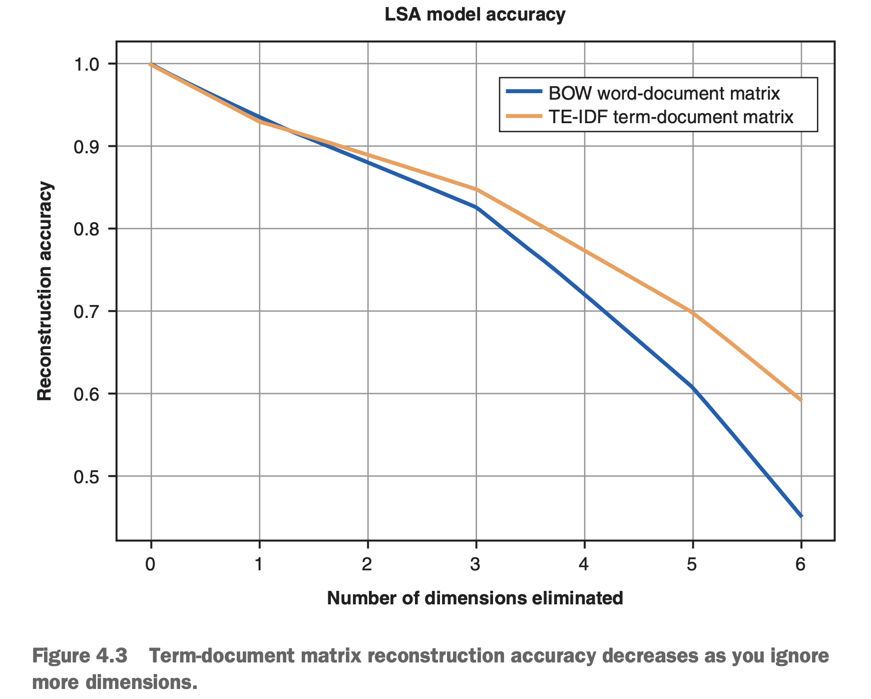
As you can see, the accuracy drop is pretty similar, whether you use TF-IDF vectors or BOW vectors for your model. But TF-IDF vectors will perform slightly better if you plan to retain only a few topics in your model.
In some cases you may find that you get perfect accuracy, after eliminating several of the dimensions in your term-document matrix. Can you guess why? The SVD algorithm behind LSA “notices” if words are always used together and puts them together in a topic. That’s how it can get a few dimensions “for free.”
Principal component analysis
Principal component analysis is another name for SVD when it’s used for dimension reduction, like you did to accomplish your latent semantic analysis earlier. And the PCA model in scikit-learn has some tweaks to the SVD math that will improve the accuracy of your NLP pipeline.
SVD maximizes the variance along each axis. And variance turns out to be a pretty good indicator of “information,” or that “essence” you’re looking for.
Original data
many dimensions
     ↓
find directions with the most variation
     ↓
keep the strongest directions
     ↓
fewer dimensions
but most useful information remains
Instead of representing a document with thousands of word dimensions, PCA/SVD can represent it with a much smaller number of latent dimensions while preserving much of the structure in the original data.
10,000 word dimensions
        ↓
PCA / SVD
        ↓
100 latent dimensions
Dimension reduction is the primary countermeasure for overfitting. By consolidating your dimensions (words) into a smaller number of dimensions (topics), your NLP pipeline will become more “general.” Your spam filter will work on a wider range of SMS messages if you reduce your dimensions, or “vocabulary.”
That’s exactly what LSA does—it reduces your dimensions and therefore helps prevent overfitting.
Whichever algorithm or implementation you use for semantic analysis (LSA, PCA, SVD, truncated SVD, or LDiA), you should normalize your BOW or TF-IDF vectors first. Otherwise, you may end up with large scale differences between your topics.
SVD use cases:
TF-IDF / BOW sparse matrix
        ↓
TruncatedSVD
        ↓
LSA / topic vectors
PCA use cases:
Dense numeric data
        ↓
PCA
        ↓
lower-dimensional representation
PCA is usually better for dense, centered numeric data. TruncatedSVD is usually better for sparse NLP matrices such as TF-IDF. Both reduce dimensions by keeping the directions that preserve the most useful variation in the data.
Latent Dirichlet allocation (LDiA)
LSA should be your first choice for most topic modeling, semantic search, or content-based recommendation engines.38 Its math is straightforward and efficient, and it produces a linear transformation that can be applied to new batches of natural language without training and with little loss in accuracy. But LDiA can give slightly better results in some situations.
LDiA, Infer which topics exist in a corpus, which words belong strongly to each topic, and what mixture of topics makes up each document. All of this is made with a probabillistic model.
Steps:
- Start with documents ↓
- Convert them to Bag-of-Words counts ↓
- Choose number of topics K ↓
- LDiA learns which words belong to each topic ↓
- LDiA computes the topic mixture for each document ↓
- Each document becomes a topic vector
Key difference from SVD/SLA
LSA / SVD finds linear combinations of words that capture maximum variance
LDiA models documents probabilistically as mixtures of topics made of distributions of words
Also, topic selection by LDiA is more friendly for humans.
This is because words that frequently occur together are assigned the same topics, and humans expect that to be the case. Where LSA (PCA) tries to keep things spread apart that were spread apart to start with, LDiA tries to keep things close together that started out close together.
This may sound like it’s the same thing, but it’s not. The math optimizes for different things. Your optimizer has a different objective function so it will reach a different objective. To keep close high-dimensional vectors close together in the lowerdimensional space, LDiA has to twist and contort the space (and the vectors) in nonlinear ways. This is a hard thing to visualize until you do it on something 3D and take “projections” of the resultant vectors in 2D.
LDiA works with raw BOW count vectors rather than normalized TF-IDF vectors.
BOW counts:
Vocabulary:
[cat, dog, city, apple]
Doc 1: “cat cat dog” Doc 2: “city apple city” Doc 3: “cat city”
cat dog city apple
Doc 1 2 1 0 0 Doc 2 0 0 2 1 Doc 3 1 0 1 0
Vectors:
Doc 1 = [2, 1, 0, 0] Doc 2 = [0, 0, 2, 1] Doc 3 = [1, 0, 1, 0]
Interpretation:
2 = word appears twice 1 = word appears once 0 = word does not appear
Normalized TF-IDF vectors:
cat dog city apple
Doc 1 0.74 0.67 0.00 0.00 Doc 2 0.00 0.00 0.74 0.67 Doc 3 0.71 0.00 0.71 0.00
As vectors:
Doc 1 = [0.74, 0.67, 0.00, 0.00] Doc 2 = [0.00, 0.00, 0.74, 0.67] Doc 3 = [0.71, 0.00, 0.71, 0.00]
Now the values no longer mean:
“how many times did this word appear?”
They mean more like:
“how important is this word in this document, relative to the rest of the corpus?”
Distance and similarity
Remember that you can use similarity scores (and distances) to tell how similar or far apart two documents are based on the similarity (or distance) of the vectors you used to represent them.
LSA preserves large distances, but it doesn’t always preserve close distances (the fine “structure” of the relationships between your documents). The underlying SVD algorithm is focused on maximizing the variance between all your documents in the new topic vector space.
sklearn.metrics.pairwise module

'cityblock', 'cosine', 'euclidean', 'l1', 'l2', 'manhattan', 'braycurtis',
'canberra', 'chebyshev', 'correlation', 'dice', 'hamming', 'jaccard',
'kulsinski', 'mahalanobis', 'matching', 'minkowski', 'rogerstanimoto',
'russellrao', 'seuclidean', 'sokalmichener', 'sokalsneath', 'sqeuclidean',
'yule'
Steering with feedback
Steering with feedback means using labels, user judgments, or metadata to adjust vector positions or distance metrics so that useful pairs move closer together and bad pairs move farther apart.
Topic vector power
With topic vectors, you can do things like compare the meaning of words, documents, statements, and corpora. You can find “clusters” of similar documents and statements. You’re no longer comparing the distance between documents based merely on their word usage. You’re no longer limited to keyword search and relevance ranking based entirely on word choice or vocabulary. You can now find documents that are relevant to your query, not just a good match for the word statistics themselves.
Semantic search
When you search for a document based on a word or partial word it contains, that’s called full text search. This is what search engines do. They break a document into chunks (usually words) that can be indexed with an inverted index like you’d find at the back of a textbook. It takes a lot of bookkeeping and guesswork to deal with spelling errors and typos, but it works pretty well.
Semantic search is full text search that takes into account the meaning of the words in your query and the documents you’re searching. In this chapter, you’ve learned two ways— LSA and LDiA—to compute topic vectors that capture the semantics (meaning) of words and documents in a vector. One of the reasons that latent semantic analysis was first called latent semantic indexing was because it promised to power semantic search with an index of numerical values, like BOW and TF-IDF tables. Semantic search was the next big thing in information retrieval.
Summary:
- You can use SVD for semantic analysis to decompose and transform TF-IDF and BOW vectors into topic vectors.
- Use LDiA when you need to compute explainable topic vectors
- All vector can perform semantic search based on their meaning
- Topic vectors can be used to predict whether a social post is spam
- to sidestep around the curse of dimensionality to find approximate nearest neighbors in your semantic vector space. tools: https://github.com/spotify/annoy https://radimrehurek.com/gensim/models/keyedvectors.html
Details
- Natural Language Processing in Action: Understanding, analyzing, and generating text with Python by Hobson Lane, Cole Howard & Hannes Max Hapke
- ISBN: 9781617294631 (look up with WorldCat, Open Library, or buy locally with IndieBound)
- Published: 2019
- Publisher: Manning